6  Good Coding Practices

Summary

In the last chapters, you have learned how to name your names and variables and how to set up an organized project structure. In this chapter, you will learn good coding practices to help other researchers and your future self with the code you used for your analysis.

6.1 R projects

As a researcher (and as a student), you work on different projects simultaneously. You have different research projects and teaching parts that you need to cover in your job. You attend different courses and give presentations and perform data analyses in these seminars and lectures. As you learned in the previous chapter about project structure, it makes sense to set up your files and folders in a particular research project folder.

Output

projects/
├── version-control-book
├── reproducibility-book
├── grant_neuroscience_horizon
├── grant_neuroscience_dfg

We highly recommend to use specific R-projects for each project, respectively. This will become clear throughout this chapter and the next chapter about renv.

To create an R-project, follow these steps:

1. Open RStudio.
2. Click on the blue cube with a in it and a green plus on the outside.
3. Decide whether you want to create a new directory or an existing directory.

Depending on your situation, it makes sense to either create a new directory or turn an existing folder into an R project.
When you are at the beginning of your project and have not set up a project structure yet, it makes sense to create a new directory.
Make sure that, in this case, your directory name aligns well with your project.
When you have already set up a project structure, it makes sense to turn your project folder into an R project. Make sure that, in this case, your project folder is the folder you turn into an R project.

New directory

Click on New Directory, then New Project, and type in your directory name.
Make sure that your project is in the correct place in your folder system.
At this point, it does not matter whether you want to create a Git repository and/or use renv with this project.
In future chapters, you will learn the advantages of using Git and renv.

When you click on Create Project, your R project will be created.
You will see that R has created a folder named after your directory and that one file, directory-name.Rproj, is in this folder.

Existing directory

Click on Existing Directory and make sure which folder you want to turn into an R project.

When you click on Create Project, your R project will be created. You will see that R has placed a file in your chosen folder called directory-name.Rproj.

What is an .Rproj-file?

The .Rproj file contains settings for all files associated with your specific R project.
It is automatically created when you set up an R project. By double-clicking on the file, you can open the project in RStudio.
It is not recommended to modify this file manually.

After you have created your R project, it is time to take a closer look at your R scripts containing the code for your projects.

6.2 Comments

Comments are probably the most important part of your scripts (but also see the discussion in Tip 6.1). Whenever you write a # in your R-script, all code after that # will be identified as comment and therefore not be executed as code. Thus, if you put a # at the beginning of a line, the whole line will be identified as comment. Here are some thoughts about comments by Rennie (2024):

Adding comments

• Add comments using a # in R (in a separate line)
• Comments don’t need to explain what your code does
• Comments should explain why you did it

You can use # not only for comments but also for creating sections and subsections in your R-script. To do so, you must start a line with at least one hash # and put at least 4 hyphens after your comment. The number of hashes you use at the beginning determines the level of section.

Code

# Section 1 ----

## Subsection 1.1 ----

## Sebsection 1.2 ----

# Section 2 ----

Tip 6.1: Discussion: Pros and cons of comments

Comments in code are useful because they help explain complex logic, provide context for why certain decisions were made, and assist future developers in understanding the code faster.

However, ideally, code should be written clearly enough that its purpose and functionality are apparent without the need for excessive comments. Well-structured, self-explanatory code enhances readability and reduces maintenance.

On the other hand, beginners often find comments valuable, even in well-written code, as they can serve as a learning tool, guiding them through unfamiliar concepts and helping them understand the underlying logic.

6.3 File paths

Whenever you are conducting research, you need to analyze some form of data. This data is typically stored in one or more files. Therefore, you need to read the data into your script. To do so, you must refer to the files you want to read. This is where the first advantage of setting up a dedicated R project for your research becomes apparent.

You can read data or code into your R environment by referring to your files using absolute paths, relative paths, and here::here().

6.3.1 Absolute paths

Using an absolute path means referring to your file by specifying the entire folder structure on your computer:

Code

data <- read_csv("/Users/my-user-name/Documents/projects/my-project/data/data-raw.csv")

Using absolute file paths is not recommended for computational reproducibility.
A collaborator or interested researcher who downloads your scripts and wants to reproduce your analysis would need to adjust these paths before the scripts can run correctly.

Code

data <- read_csv("/Users/user-name-b/Desktop/work/research/my-project/data/data-raw.csv")

6.3.2 Relative paths

A relative file path starts from your current working directory and appends the relative path.
You can check your current working directory in R by using the getwd() command in the R Console.

R Console

> getwd()
[1] "Users/my-user-name/my-project"

By default, the working directory in an R project is the project folder, which in this example is called my-project.

You can then use a relative file path from that folder to read your data.
The file path should start after the working directory:

Code

data <- read_csv("data/data-raw.csv")

Thus, all relative paths to the files in an R project remain the same, regardless of who wants to work with the project. However, this does not hold true for scripts changing the working directory using the setwd() command.

Relative file path does work

Console

> getwd()
[1] "Users/my-user-name/my-project"
> file.edit("script/script01.R")

Relative file path does not work

Console

> setwd("script")
> getwd()
[1] "Users/my-user-name/my-project/script"
> file.edit("script/script01.R")

6.3.3 The here package

A way to avoid confusion about which file paths to use is the here package (Müller 2020). The here() function works regardless of your current working directory.

You can install the here package by typing:

Code

install.packages("here")

With here::here(), it is possible to refer to file paths regardless of your working directory. here() uses the top-level directory of a project to build the paths. It recognizes special files (e.g., .Rproj) and infers the project folder. Using here(), referencing file paths will always follow the same project structure regardless of the file you are referencing.

Example

here() function works regardless of the current working directory.

No change in working directory

Console

getwd()
[1] "/Users/my-user-name/my-project"
> here()
[1] "/Users/my-user-name/my-project"
> source(here("scripts", "script01.R"))

Change in working directory

Console

getwd()
[1] "/Users/my-user-name/my-project"
> here()
[1] "/Users/my-user-name/my-project"
> source(here("scripts", "script01.R"))

Another benefit of using here() is enhanced readability because the paths always start at the project directory. Using relative paths would require the reader to consider the current working directory and how certain files are relatively located to it. Furthermore, here() remains unaffected by differences between operating systems when separating files with characters and commas.

Path differences between operating systems

macOS and Linux use a slash / for path separators, while Windows uses a backslash \. In R, \ is an escape operator, causing R to misinterpret Windows backslashes \ when used as path separators. On Windows, using \\ or / is necessary to handle path separators correctly.

A benefit of here() is that paths can be specified within "" and separated by commas. Depending on the operating system, here() applies the correct path separator automatically.

Code

source(here("folder", "subfolder", "subsubfolder", "file.R"))

In summary, we recommend using the here::here() function because it is most robust against different paths. Relative file paths can also work if the working directory does not change in one of the project scripts and only / are used for path specifications. We recommend to never use absolute file paths, since they are a hurdle to computational reproducibility.

6.4 Code Style

“Good coding style is like correct punctuation: you can manage without it, butitsuremakethingseasiertoread” – Wickham, Çetinkaya-Rundel, and Grolemund (2023)

One important aspect that fosters understandability of code is the code style. In this section, we will present the tidyverse-codestyle (Wickham, Çetinkaya-Rundel, and Grolemund 2023). The Tidyverse is a collection of R packages particularly useful for data wrangling, manipulation and visualization. All packages share an underlying design philosophy, grammar, and data structures.

In psychology, the grammar of the tidyverse is widely used for data wrangling. In this section, we will provide a brief introduction to code style.

6.4.1 Names

Not only should files and folders be named well (see chapter on naming things), but the same applies to variable and function names in scripts. Variable and function names should only consist of lowercase letters, numbers, and underscores (_). It is better to use descriptive, longer names rather than short abbreviations that you may not understand in the future.

Strive for

short_flights <- flights |>
  filter(air_time < 60)

Avoid

SHORTFLIGHTS <- flights |>
  filter(air_time < 60)

6.4.2 Spaces

Put spaces around mathematical operators (except ^) and around the assignment operator (<-). Do not put spaces around parentheses when using functions. Put a space after a comma, as you would in standard English.

Strive for

mean(x, na.rm = TRUE)

Avoid

mean (x ,na.rm=TRUE)

6.4.3 Pipes

The pipe (either |> or %>%) is a useful operator for connecting subsequent operations in your code. The pipe takes everything to the left of it and uses it as the first argument to the function on the right side.

Without pipe

sum(c(1:4))

With pipe

c(1:4) |> sum()

The pipe is particularly useful when you chain many functions together. Therefore, use |> at the end of a line and add a space before it. The complete sequence of functions connected by a pipe is also called a pipeline.

Strive for

data |>
  select(N, gender) |>
  filter(
    gender == "male" |
    gender == "female"
  ) |>
  group_by(gender) |>
  summarise(
    mean = mean(N),
    median = md(N)
  )

1

Take the data and then

2

Select the variables N and gender and then

3

Filter all observations where the variable gender either contains the value male or female and then

4

Group the dataset by the variable gender and then

5

Summarize your datasets by calculating the mean and median for the variable N for each group.

Avoid

summarise(group_by(filter(select(data, N, gender), gender == "male" | gender == "female"), gender), mean = mean(N))

The code displayed above is much easier to read and understand for your future self and other researchers, thereby increasing the likelihood of reproducibility. Translated into plain English, the pipe represents an “and then”:

Difference between %>% and |>

In basic code, %>% and |> behave the same in the simple cases we cover here. In general, %>% has some advantages when you want to code more complex cases. If you are interested when it matters if you either use %>%or |>, we recommend this resource.

%>%

The %>% pipe was introduced in the context of the tidyverse. It comes with the package magrittr and con only be used when this package is installed and loaded.

Code

install.packages("magrittr")
library(magrittr)

However, you can also use it, when you load another package from the tidyverse such as dplyr. This is because dplyr imports magrittr when it is loaded.

|>

The |> pipe comes with the basic R. To use |> in R, you have to go to Tools > Global Options > Code and tick the box Use native pipe operator, |> (repquires R 4.1+).

6.4.4 Line breaks

If a function requires you to name arguments (as with summarise()), put each argument on a new line. If a function does not require you to name arguments (as with group_by()), keep your code on one line unless it extends beyond the width of a line. In that case, put each argument on its own line.

When you start a new line after using |> or a function like summarise(), indent the new line by two spaces (if not already done automatically). If you are putting each argument on a separate line, also indent the new line by two spaces. Make sure that the closing parenthesis ) is on its own line and not indented. Thus, the closing parenthesis should align with the horizontal position of the function you are using.

Strive for

flights |>  
  group_by(tailnum) |> 
  summarize(
    delay = mean(
      x = arr_delay,
      na.rm = TRUE
    ),
    n = n()
  )

Avoid

flights|>
  group_by(tailnum) |> 
  summarize(
             delay = mean(arr_delay, na.rm = TRUE), 
             n = n()
           )

Avoid

flights|>
  group_by(tailnum) |> 
  summarize(
  delay = mean(arr_delay, na.rm = TRUE), 
  n = n()
  )

6.4.5 Evaluate your code style: Linting

After learning the tidyverse coding style, you can check your code for any deviations from that style.
This process is called “linting” and is comparable to a program that checks for spelling errors.
The lintr package (Hester et al. 2024) can perform this task by analyzing your code for potential issues and deviations from the recommended coding style.

• stylistic issues (e.g. x<-3 vs. x <- 3)
• common errors (e.g. mean(x, na.rm = T, na.rm = F))
• missing packages
• …

Caution

However, note that lintr cannot check whether your code runs correctly!

Example of lintr

Suppose you have script called test-script.R in the folder scripts of your research projects. Your script looks as follows:

Script

# Test Script

df <- matrix(c(1,2,3,4,5,6), nrow = 2, ncol = 3)

After you installed and loaded the package lintr, run: lintr::lint("scripts/test-script.R") in your R-console:

Code

install.packages("lintr")
library(lintr)
lintr::lint("scripts/test-script.R")

Next to your Console, a new tab will open called Markers, displaying all syntax messages lintr found in your script.

Markers

Line 3 [commas_linter] Commas should always have a space after.
Line 3 [commas_linter] Commas should always have a space after.
Line 3 [commas_linter] Commas should always have a space after.
Line 3 [commas_linter] Commas should always have a space after.
Line 3 [commas_linter] Commas should always have a space after.

In test-script.R, lintr wants us to separate the numbers 1 to 6 by spaces after commas. For every missing comma, lintr displays a separate error message. After adding the spaces, saving the script, and running lintr::lint("scripts/test-script.R") again, no error messages are displayed in the Markers tab.

6.5 Tidy Data

Figure 6.1: “Illustration from the Openscapes blog Tidy Data for reproducibility efficiency and collaboration” by Julia Lowndes and Allison Horst (License: CC-BY 4.0; reused without modifications)

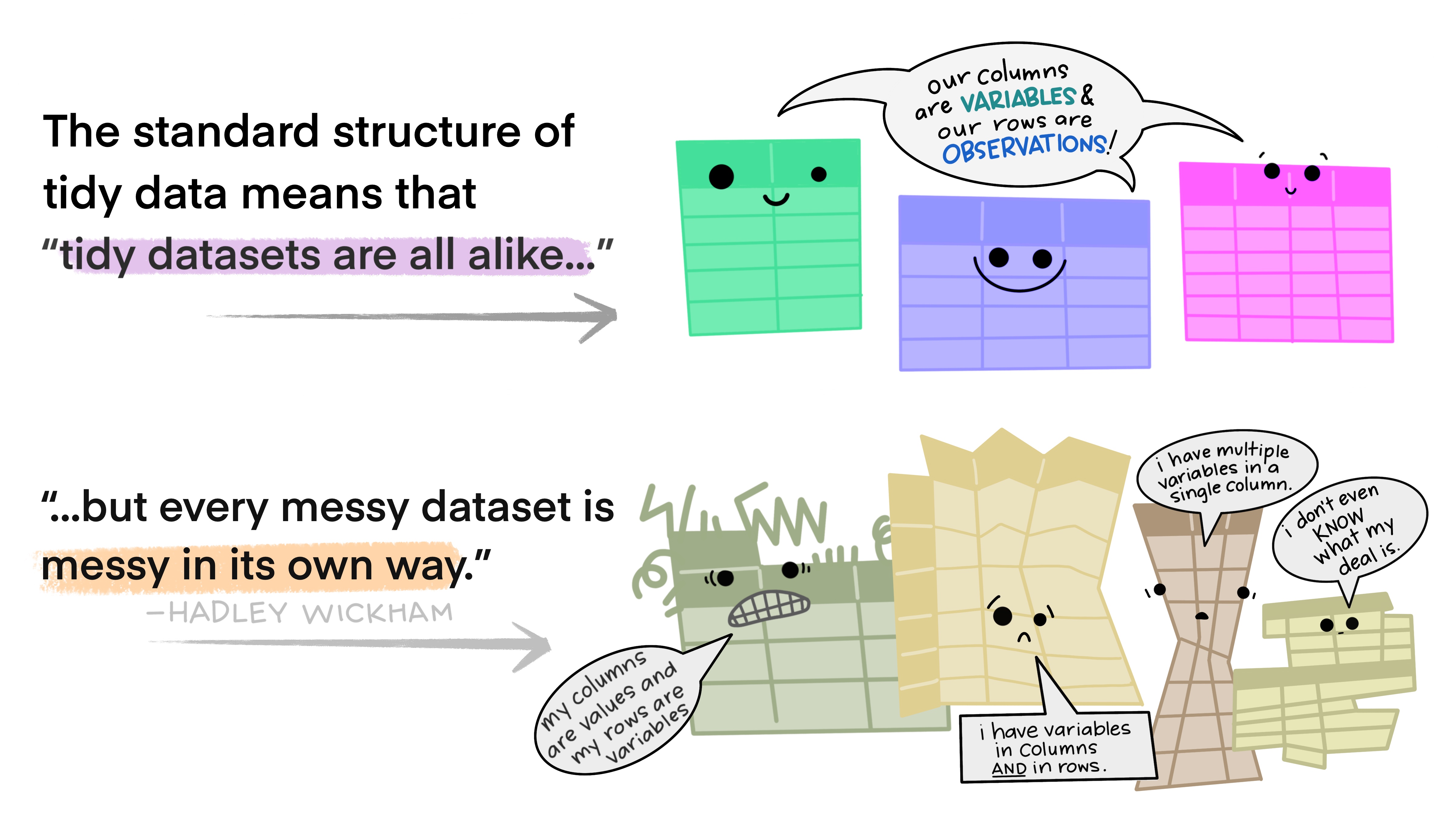
When working with datasets, you will likely not be able to directly conduct your data analysis (e.g., t-tests, ANOVAs, GLMs). In fact, most of the time, you will spend more time organizing your data than running your analysis. A helpful concept is tidy data, which is a common guideline for organizing datasets. Tidy data is closely related to the principles of the tidyverse introduced in Section 6.4. Following tidy data guidelines will help you run analyses and get the most out of your data.

Tidy Data

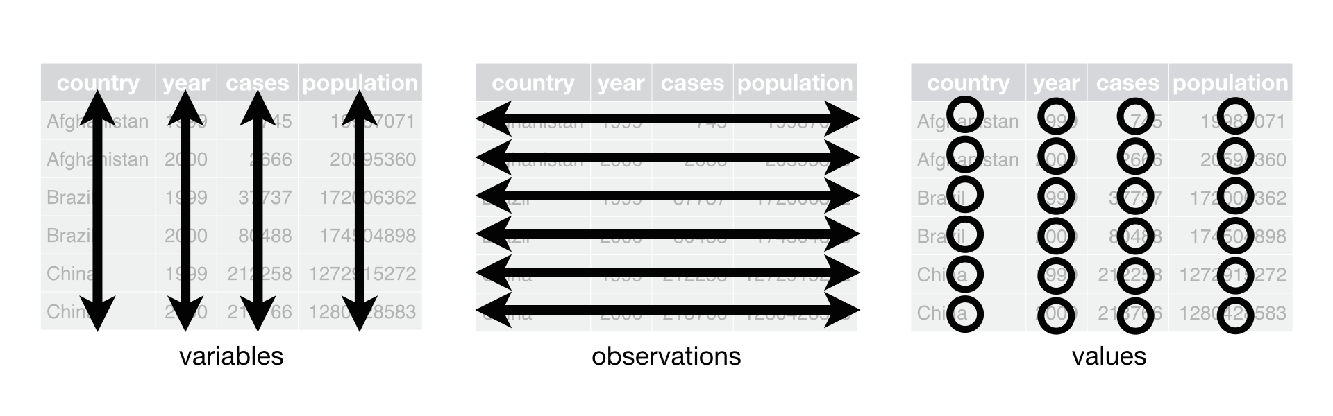
Tidy datasets follow three basic rules:

1. Each variable is a column, and each column is a variable.
2. Each observation is a row, and each row is an observation.
3. Each value is a cell, and each cell contains a value.

Figure 6.2: “Tidy Data” by Hadley Wickham and Mine Çetinkaya-Rundel and Garret Grolemund (License: CC BY-NC-ND 3.0 US; reused without modifications)

The journey from raw to tidy data can be long and frustrating. This book cannot provide a full overview of data wrangling and manipulation. However, if you are interested in learning functions for data manipulation, we recommend studying the dplyr package and its documentation, as well as the tidyr package and its documentation. From our experience, using and sharing code written in the tidyverse style fosters better understanding of the code, thereby enhancing computational reproducibility.

6.5.1 Data structures

Data can be structured in different ways. When your data is tidy, you may still encounter wide or long formats. As a rule of thumb, you can remember this: Data structured in a long format usually contains repetitive values in the first column of the dataset. Data structured in a wide format usually contains non-repetitive values in the first column of the dataset.

Wide format

# A tibble: 3 × 3
  participant congruent incongruent
        <int>     <dbl>       <dbl>
1           1       560         720
2           2       623         799
3           3       547         812

Long format

# A tibble: 6 × 3
  participant congruency  reaction_time
        <dbl> <chr>               <dbl>
1           1 congruent             560
2           1 incongruent           720
3           2 congruent             623
4           2 incongruent           799
5           3 congruent             547
6           3 incongruent           812

However, this rule of thumb does not always apply, for example when data is rearranged.

[1] "Data in long format"

# A tibble: 6 × 3
  reaction_time congruency  participant
          <dbl> <chr>             <dbl>
1           560 congruent             1
2           720 incongruent           1
3           623 congruent             2
4           799 incongruent           2
5           547 congruent             3
6           812 incongruent           3

Another perspective on wide vs. long data comes from the context of the data. In research, a common question is how variable A influences variable B. Variable B is dependent on variable A, making variable B the dependent variable (DV) and variable A the independent variable (IV).

In the wide data format, the names of the factor levels of the IV are usually column names, while the DV is displayed as the values across these cells. In contrast, in the long data format, the names of the factor levels of the IV are typically values in the column of the IV. The name of the IV becomes the column name, rather than the level of the IV. Simultaneously, the DV is displayed in one column with the name of the DV as the column name and the corresponding values in that column.

6.5.2 Changing the data structure

Depending on which R functions you want to use or other reasons, you may need to or want to change your data structure from wide to long or vice versa. An easy way to do this is by using pivot_wider() and pivot_longer() from the tidyr package.

6.5.2.1 pivot_longer()

pivot_longer() takes your dataset and makes it longer. It takes certain columns and places their names as values into a new column. Additionally, it combines the values of these columns into a single column.

Code

library(tidyr)
data_wide |>
  pivot_longer(
    cols = c("congruent", "incongruent"),
    names_to = "congruency",
    values_to = "reaction_time"
  )

1

Take the dataset data_wide, then

2

Apply the function pivot_longer() to the data by

3

Specifying the columns that should be transformed into a long format,

4

Naming the new column to hold the previous column names, and

5

Naming the new column to hold the values of the previous columns.

# A tibble: 6 × 3
  participant congruency  reaction_time
        <int> <chr>               <dbl>
1           1 congruent             560
2           1 incongruent           720
3           2 congruent             623
4           2 incongruent           799
5           3 congruent             547
6           3 incongruent           812

6.5.2.2 pivot_wider()

pivot_wider() takes your dataset and makes it wider. It takes the names of a certain column and changes them to new column names. Further, it takes the values of a second column and puts them across the new columns to their corresponding names.

Code

data_long |>
  pivot_wider(
    names_from = "congruency",
    values_from = "reaction_time"
  ) |>
  print()

1

Take the dataset data_long,

2

Apply the function pivot_wider() to the data by

3

Specifying the column name from which to create the new column names, and

4

Specifying the column name from which to take the values for the new columns.

# A tibble: 3 × 3
  participant congruent incongruent
        <dbl>     <dbl>       <dbl>
1           1       560         720
2           2       623         799
3           3       547         812

6.6 Defensive programming

Whenever you write code for data analysis or any other purpose, it is useful to validate what you are doing. This is also known as defensive programming. “Defensive” in this context means cautious. Here are some potential benefits of validating your code:

• Early error detection
  
• Code clarity
  
• Protection against invalid input
  
• Monitoring data quality
  
• Improved documentation
  
• Improved error handling

6.6.1 The assertr package and it’s function verify()

The assertr package helps you when you start testing your code. Once you begin adopting the tidyverse coding style, the function verify() will be easy to apply in your code. verify() can be seamlessly integrated into a code pipeline.

The verify() function takes a data frame (which is the first argument of the function and provided by the |> operator) and a logical expression. Then, the expression is evaluated in the context of the data frame. When the expression is TRUE, no error occurs and the pipe goes on. When the expression is FALSE, verify will raise an error that terminates any further processing of the pipeline (Fischetti 2023).

Verification passed

In this example, a dataframe will only be printed, if all values in the column reaction_time are higher than 200. This holds true for data_long, but not for data_long_2. data_long_2 has one value (24) violating the verify expression.

Code

library(assertr)

# verify if reaction time is longer than 200ms
data_long |>
  verify(reaction_time > 200) |>
  print()

# A tibble: 6 × 3
  participant congruency  reaction_time
        <dbl> <chr>               <dbl>
1           1 congruent             560
2           1 incongruent           720
3           2 congruent             623
4           2 incongruent           799
5           3 congruent             547
6           3 incongruent           812

Verification failed

In this example, a dataframe will only be printed, if all values in the column reaction_time are higher than 200. This holds true for data_long, but not for data_long_2. data_long_2 has one value (24) violating the verify expression.

Code

data_long_2 <- data_long
data_long_2[5,3] <- 24

data_long_2 |>
  verify(reaction_time > 200) |>
  print()

Console output

verification [reaction_time > 200] failed! (1 failure)

    verb redux_fn           predicate column index value
1 verify       NA reaction_time < 200     NA     5    NA

Error: assertr stopped execution

6.6.2 Further functions and packages

The verify() function provides an easy way to start validating your code within a tidyverse coding style. However, there are more functions from the assertr package that can be applied for defensive programming. Going through all of these functions exceeds the scope of this book. Therefore, we highly recommend reading the accompanying vignette by Tony Fischetti, the author of the assertr package.

Furthermore, assertr is not the only package dealing with defensive programming. assert, assertthat, and testthat are other powerful packages in this context. In general, code validation is not too popular in scientific practice. It is rather prevalent in software development contexts validating functions and whole scripts for specific purposes. These thorough testing processes extends the scope of computational reproducibility in our opinion. Thus, we recommend assertr::verify() as a good starting point for defensive programming in the context of computational reproducibility.

6.7 Acknowledgements & further reading

We would like to express our gratitude to the following resources, which have been essential in shaping this chapter. We recommend these references for further reading:

Resources
(Rennie 2024)
(Wickham, Çetinkaya-Rundel, and Grolemund 2023)

Fischetti, Tony. 2023. Assertr: Assertive Programming for r Analysis Pipelines. https://doi.org/10.32614/CRAN.package.assertr.

Gorgolewski, Krzysztof J., Tibor Auer, Vince D. Calhoun, R. Cameron Craddock, Samir Das, Eugene P. Duff, Guillaume Flandin, et al. 2016. “The Brain Imaging Data Structure, a Format for Organizing and Describing Outputs of Neuroimaging Experiments.” Scientific Data 3 (1). https://doi.org/10.1038/sdata.2016.44.

Hester, Jim, Florent Angly, Russ Hyde, Michael Chirico, Kun Ren, Alexander Rosenstock, and Indrajeet Patil. 2024. Lintr: A ’Linter’ for r Code. https://CRAN.R-project.org/package=lintr.

Müller, Kirill. 2020. Here: A Simpler Way to Find Your Files. https://here.r-lib.org/.

Rennie, Nicola. 2024. “Writing Better r Code.” https://nrennie.rbind.io/training-better-r-code/.

Wickham, H., M. Çetinkaya-Rundel, and G. Grolemund. 2023. R for Data Science: Import, Tidy, Transform, Visualize, and Model Data. O’Reilly Media. https://r4ds.hadley.nz.