YAML
---
editor:
  markdown:
    wrap: sentence
---In this chapter you will learn how you can automatically integrate your reproducible results into a paper. You will learn the basics of Markdown syntax, how to write a paper within Quarto, and how to format it for a required output. You will learn how to use extensions, specifically the apaquarto extension to write a reproducible paper in APA-style.
Imagine you are writing a paper. You have learned a lot about reproducibility (even perhaps in this book), you like the idea, and you want to apply the standards that make your research more reproducible. You have a project structure according to your community standard, you use human and machine-readable names, you provide a lot of metadata, you track your analyses with Git, and you even set up a robust, reproducible environment for all the R packages you need for your analyses. You now want to start writing your paper, open e.g. MS Word, and start writing. At some point you write the Results section. Now you want to insert your results in your Word-Document. Some frustrating work begins, where you start to type the results of your analyses in Word. Further, you inserted the figures that visualize your findings. It took a while, but finally everything is included in that Word document – congratulations.
Happily you ask some colleagues and your supervisor to review the paper. They make some comments about your theoretical background and also about - oh gosh - your results. You did forget to filter some cases in the beginning and now you have to rerun the analysis. No problem, you smoothly got the updated results, but then you realize that you have to insert the slightly different figures and results into your Word Document. All this effort of typing the results from your R code to Word has to be done again. This can happen many times during your research process. Not only by colleagues and supervisors, but also when you found out an error by yourself. Another possibility are reviewers, when you submitted a preprint to a journal. During this process, it is very likely that you mix up some results, e.g. writing the p value of your first hypothesis to your second hypothesis. Thus, transferring results from your statistic program to a text program is an opportunity for reproducibility errors. Not because you are dumb, it is because you are human. However, there is a solution to this problem - and it is called Literate Programming.
Literate programming is a form of programming in which text and source code are in one document. It is based on the idea that a code should be easy and enjoyable to read and aimed at being understood by humans, which was called Literate Programming by Knuth (1984). Instead of writing code and later annotating it with comments, literate programming suggests to write a text in the order that a person would logically conceive it and include the code as it is explained in the text. Thus, in literate programming, text is used to make code understandable. However, the concept of literate programming was extended to the idea that the text should not support the explanation for the code but rather the code can be an explanation of the document. Thus, one can write a whole paper and uses code directly in that document to support the claims made in that document. The code in these documents are stored in chunks (see Section 9.7.1) and are executable.
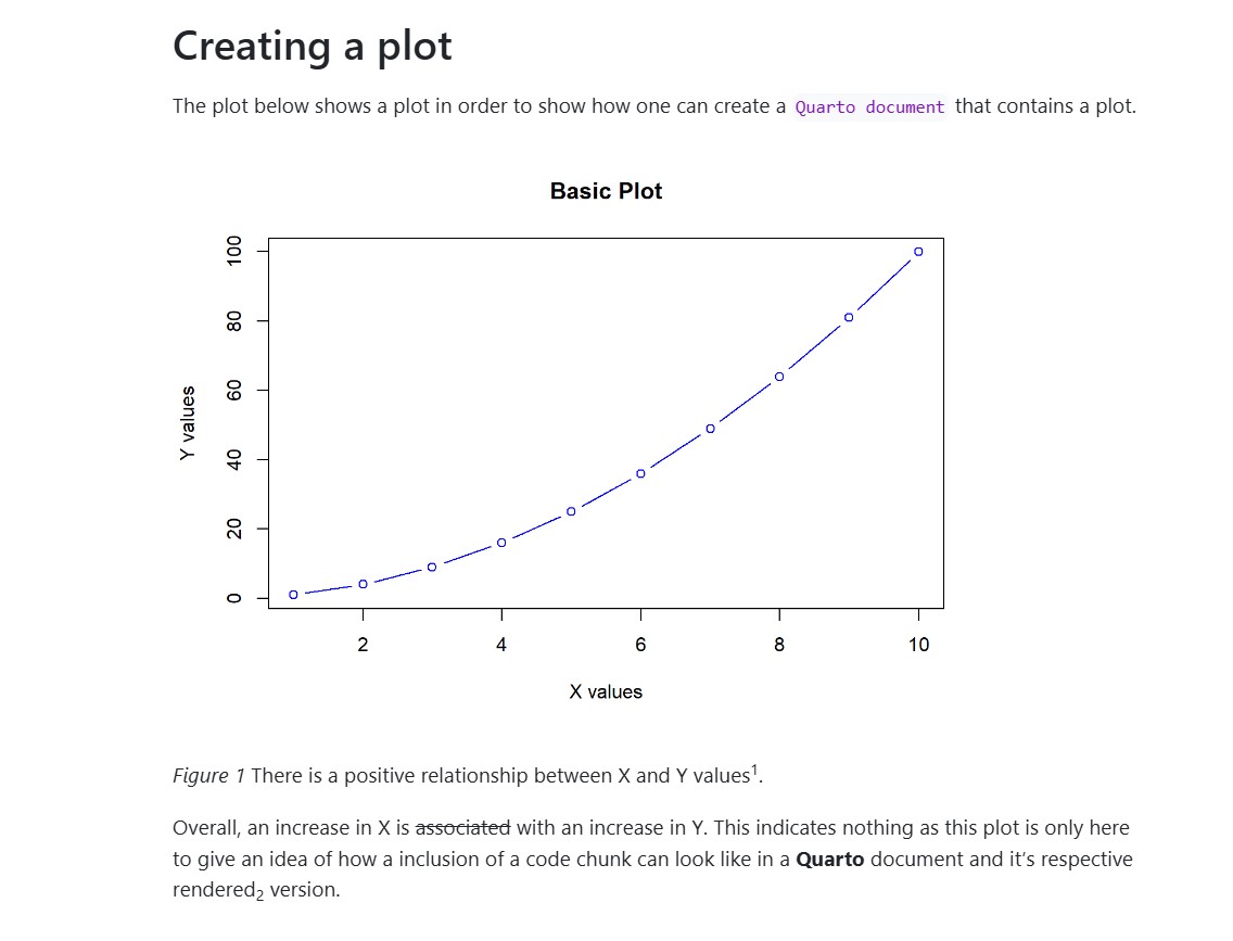
Literate programming allows for creating reproducible documents instead of just reproducible script as well as making for a smoother workflow, as there is no need for switching out old and new outputs in your documents when the code changed. As an example, when you write an article in a document using literate programming and insert a code chunk that creates a plot, this code chunk’s output (i.e. the plot) is part of your document and is always up to date with the script you’re running. Hence, whenever you have to do some changes in your plot or your analyses, the changes are directly updated in your paper. Thus, the paper becomes dynamic (Note 9.1). Moreover, literate programming can heavily reduce outcome-based reproducibility errors (Section 1.1.1).
One can discriminate static and dynamic documents. Most documents are static, since they do not refer to underlying data or content. They are typically generated once and do rarely need updates.
On the other hand, dynamic documents are generated anew if some underlying data or content changes. They are often automatically recreated and use some kind of code to generate up-to-date content. A prominent example is the dashboard of the John Hopkins University that displayed data referring to the Covid-19 Pandemic. The dashboard was updated every week with new data from all over the world.
In a classical sense, research paper can be seen as static documents, since they will be rarely updated after they were published. However, since research paper are often reviewed and many changes must be done, one can view paper as dynamic documents before publication.
Examples
| Static documents | Dynamic documents |
|---|---|
| working agreement | research paper |
| bills | dashboards |
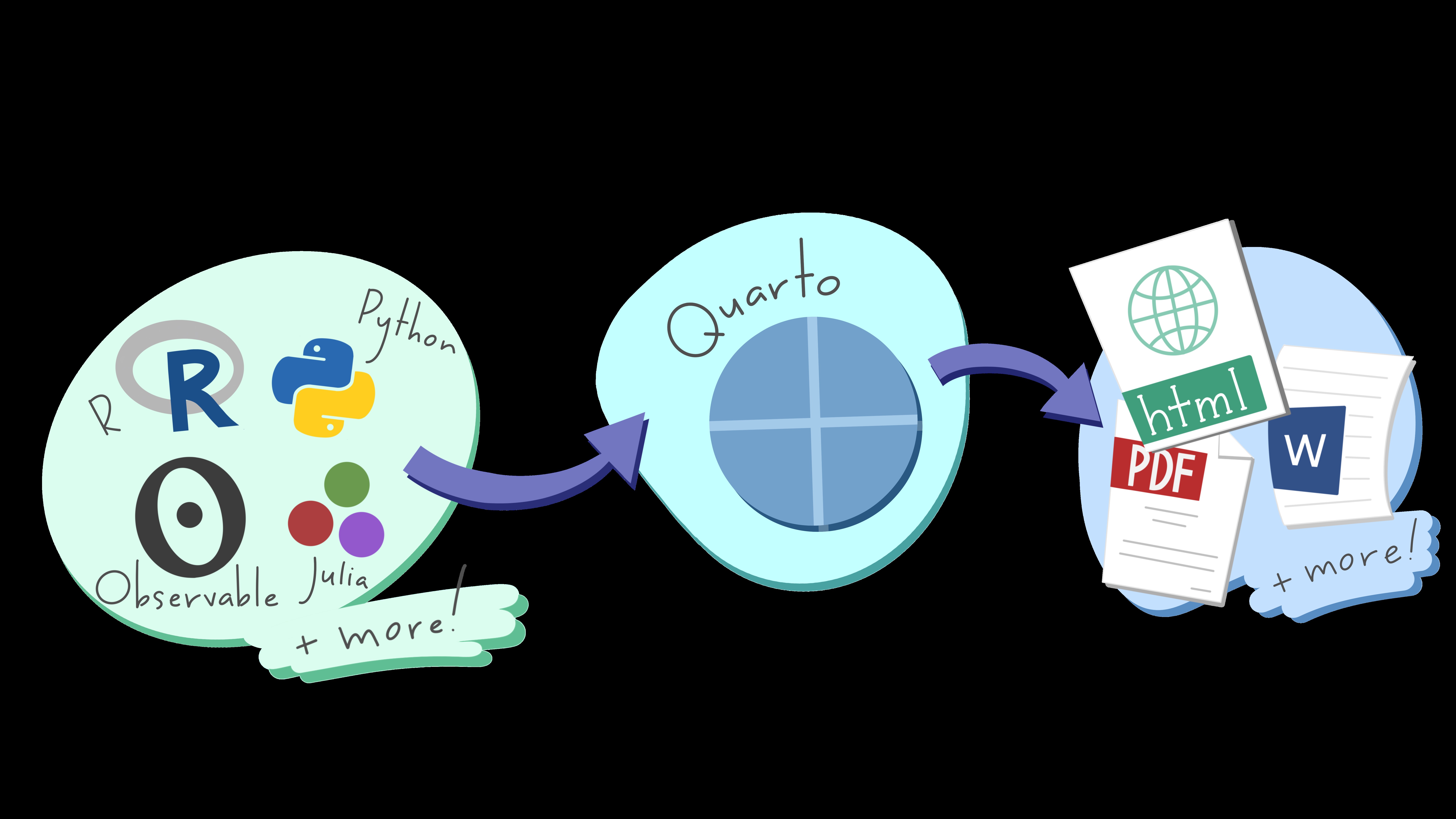
Quarto is an open-source Publishing System. It allows you to do literate programming. It was created by the company Posit, which is responsible for RStudio and is based on RMarkdown. Quarto is well integrated in RStudio and comes already bundled with any version of RStudio from RStudio v2022.07.1 “Spotted Wakerobin” onward. In case you’re using an older version of RStudio, here are instructions on how to install Quarto. What Quarto does is, it can interpret and handle many programming languages (e.g. R and Python) as well as plain text and transforms it into standard output formats (e.g., Word-, PDF-, and .html-files, see Figure 9.1).
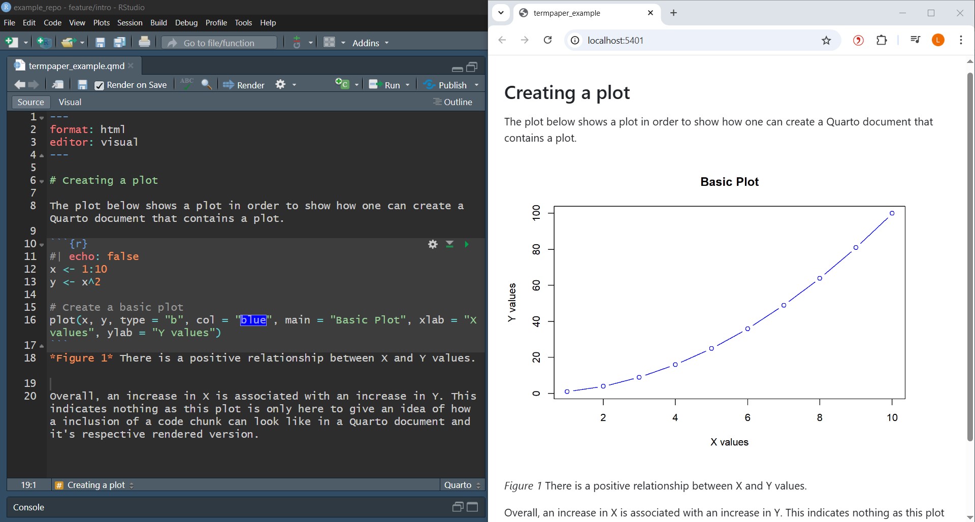
With Quarto, one is able to create (scientific) papers, but also websites, presentations or books. In fact, this book is written with Quarto. To do so, Quarto has its own file extension (.qmd). qmd stands for Quarto Markdown. We will get to the Markdown language in a second (Section 9.5). Everything you write in a Quarto file will then be rendered into a desired output file (e.g. .html, .pdf, .docx). As example, Figure 9.2 shows a Quarto document that contains human-readable text and a code chunk that will create a plot, as well as it’s rendered version below.
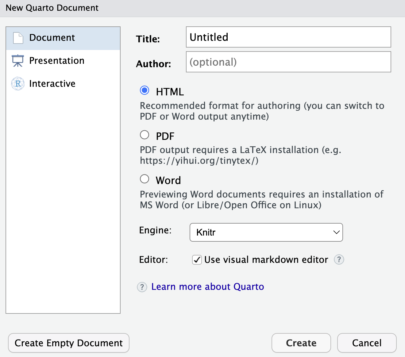
In this book, we will focus on using Quarto in RStudio, but Quarto can also be used with other editors such as VSCode or Jupyter. To start using Quarto, you must create a Quarto document. To do so, head to RStudio and in the upper left corner select File > New File > Quarto Document…. This will open a box (see Figure 9.3) that prompts you to give your document a title, which will appear at the top of your document’s rendered version, as well as choosing the format that your output will be in. Either HTML, PDF or Word are possible by default. The standard output is HTML and you do not need to have anything else installed to create html documents. If you want to create PDF or Word Documents by Quarto, you need additional software. For PDF-files, LaTeX1 is required and for Word-files, MS Word is required.
HTML files can also easily be turned into PDF files later on and the format is changeable. Depending on your project, there are other available format options as well. The metadata of title and format is stored in the so called YAML header at the top of your page. This is also where you can further customize some general features of your file, such as the author, a subtitle, the date or the style of your document (see Section 9.6). To create the Quarto document, choose your preferred output format, type in at least the title of the document, and click on Create in the prompt box.
To get a preview of a Quarto file in RStudio, you can either use quarto preview in the command line or the Render button at the top of your document. This will show you how your rendered document will look like and if you check the Render on Save box at the top of the document, will update live as you save your changes. For an example, see Figure 9.2.
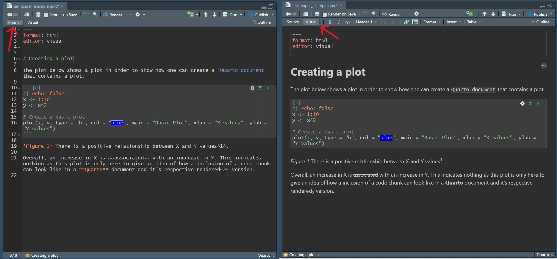
You can use either the Source or Visual mode in RStudio to write and format your work. In the Source mode you use Markdown syntax to format your written work and in the Visual mode you use a User-Interface similar to how you would use in e.g., MS Word. You can switch between the two at any time. The changes made in the Visual mode will appear in the Source mode in Markdown as well. However, we strongly recommend you to use the Source mode rather than the Visual mode. This is because most Markdown Syntax is easier and faster to write than to use a Graphical User Interface. Nevertheless, in the Section about Markdown Syntax we give you instructions how to format your text in both editors. Take a look at the two different modes and the rendered version of the document below with some simple formatting options.
Now, take a look at the rendered version of the document and how each of the formatting options plays out.
When you make changes in a Quarto document and you track it with Git, we recommend you to write each sentence in a new line when using the Source Editor. This enhances the readability of the changes in Git you made in the Quarto document but does not change the output of the document (see Figure 9.5).
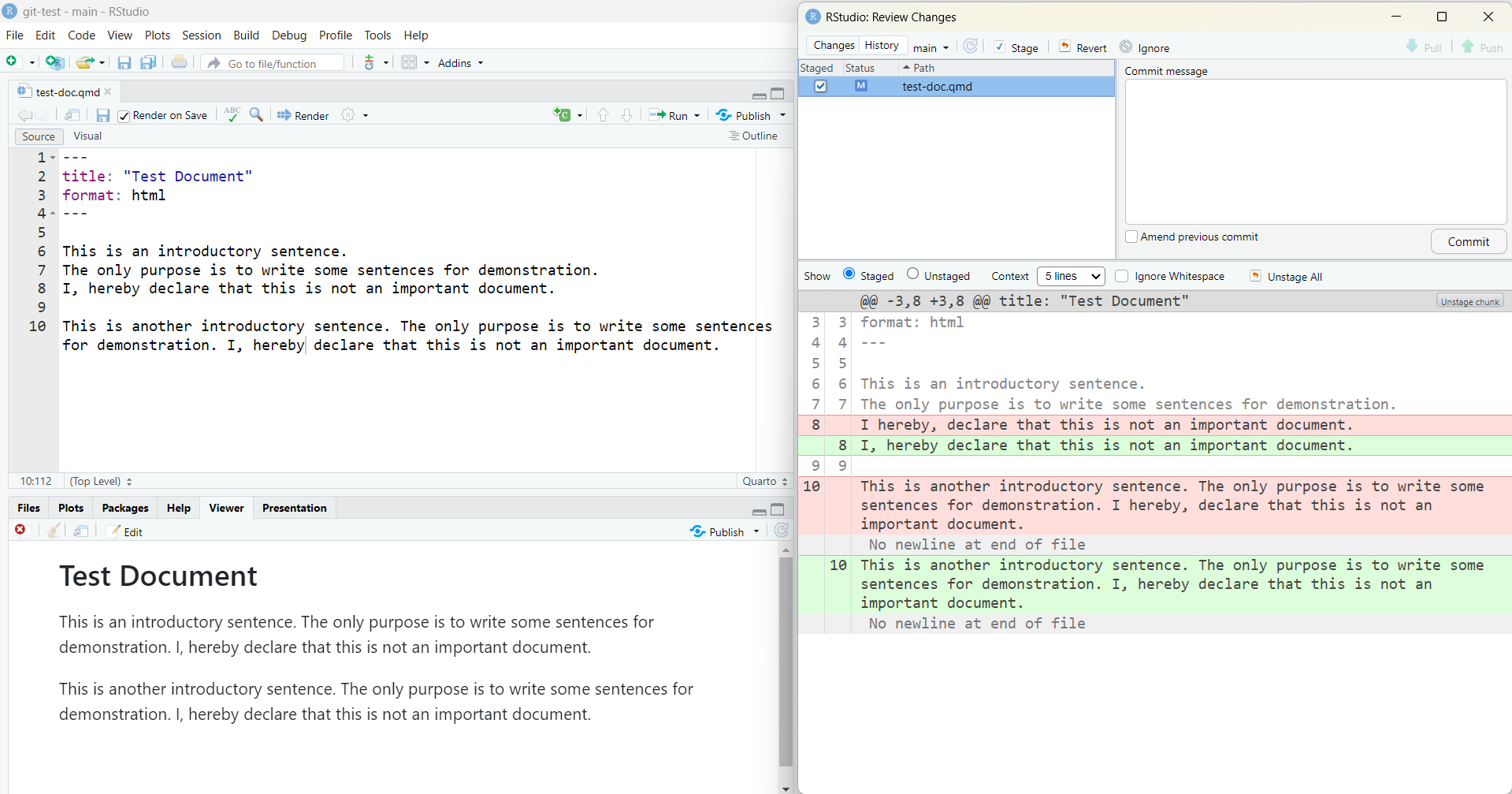
html version of the quarto document. The right half shows the popup window of Git to commit changes. As one can see, it is easier to understand the changes that were made in line 8 compared to line 10.
Source and Visual Editor
Assuming you follow Tip 9.1, and you write each sentence in a new line. When you use the Visual Editor, you are cannot directly control whether the sentences are in separate lines or not (compare Figure 9.5). However, you can specify that in the YAML header (see the code snippet below).
YAML
---
editor:
markdown:
wrap: sentence
---In Quarto documents, Markdown is used as a syntax. In Markdown content and formatting are integrated with each other and not separate. This formatting is used in Quarto or on GitHub or on a smaller scale in WhatsApp or Reddit. This formatting is different to the so-called WYSIWYG (What you see is what you get) editors, like Word. There are some advantage over these more commonly known editors. Using an integrated approach to formatting and writing allows for faster writing, as there is no need to switch between the two. You just format as you type. Another advantage is compatibility between different text editors. Any program that uses Markdown will format a document written in it the exact same way. Another advantage is that Git can track the changes made to text written with Markdown, allowing for version control of your written work the same way as of your code.
Disadvantages are that there are overall less formatting options as the intention is keep it simple and it can be difficult or unintuitive to insert tables and images.
Have a look at the different formatting options available.
When you want to format your text in the source editor, the markdown syntax is quite straightforward. For example, if you want to write italic words, you put a * around the words of interest. Table 9.1 displays how you can format your text in the most important styles.
| Input | Output |
|---|---|
*italics*, **bold**, ***bold and italics*** |
italics, bold, bold and italics |
[underlined text]{.underline} |
underlined text |
superscript^2 / subscript~2~ |
superscript2 / subscript2 |
~~strikethrough~~ |
|
`verbatim code` |
verbatim code |
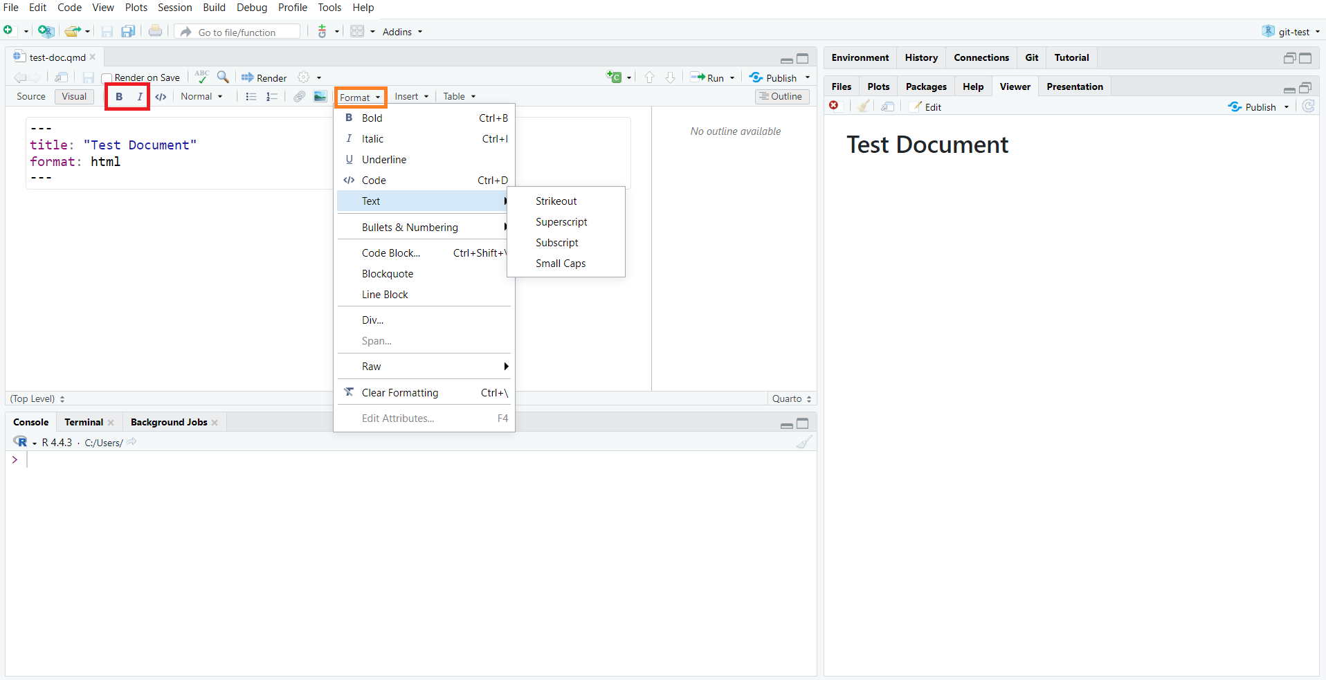
When you want to format your written text while being in the Visual Editor, you can do it by click and select. You can see a menu line at the top of the document (compare to Figure 9.6). In that line, you can just click on B to make your text bold or I to make it italic. There is also a button “Format”. If you click on that button, then a variety of formatting options appear. When you hover over “Text”, you see all the formatting options we also covered for the source editor.
If you want to start a new page in your document at a specific spot, e.g., to have your references on their own page, you can add a pagebreak. The pagebreak option does only make sense when you render your document to docx or pdf, since these files consist of multiple pages. However, this does not apply to html files, because you can just scroll down the content. To add a pagebreak, simply add it between your intended pages like below and a new page will start in the rendered document.
page 1

{{< pagebreak >}}
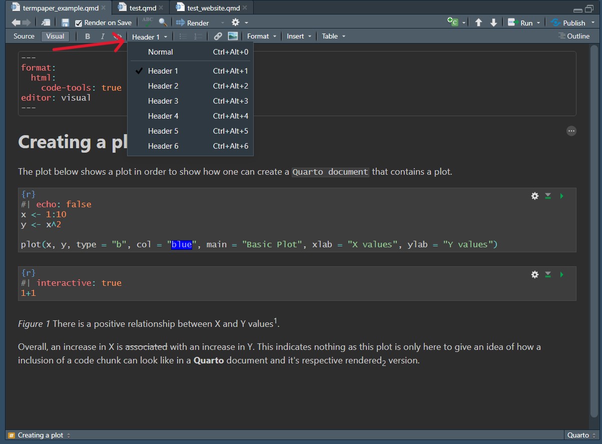
page 2Formatting headings in Markdown syntax is quite easy as well. Just put your heading in a new line, and put the number of # before that heading to indicate the heading level. The more #, the smaller the heading. You can also format your headings in the Visual Editor. However, it is faster in our experience to use the Source editor.
|
Input |
Output |
|---|---|
|
|
Header 1 |
|
|
Header 2 |
|
|
Header 3 |
|
|
Header 4 |
|
|
Header 5 |
|
|
Header 6 |
You can also edit your headings in the menu line of the Visual Editor via click and select. Simply choose between normal text or your desired header level.
There are many different types of lists available in Markdown and they are very easy to implement in Source Mode. Take a look below at the different options and how they change when rendered.
Input
*Unordered list*

* unordered list
        + sub-item 1
        + sub-item 2

*Ordered list: Standard numbering*

1. ordered list
2. item 2
  1. sub-item 1

*Ordered list: All 1:*

1. ordered list
1. item 2
1. item 3
1. item 4

*Tasklist*

- [ ] Task 1
- [ ] Task 2
Output
Unordered list
Ordered list: Standard numbering
Ordered list: All 1:
Tasklist
💡 The tasklist can be ticked off. Try it.
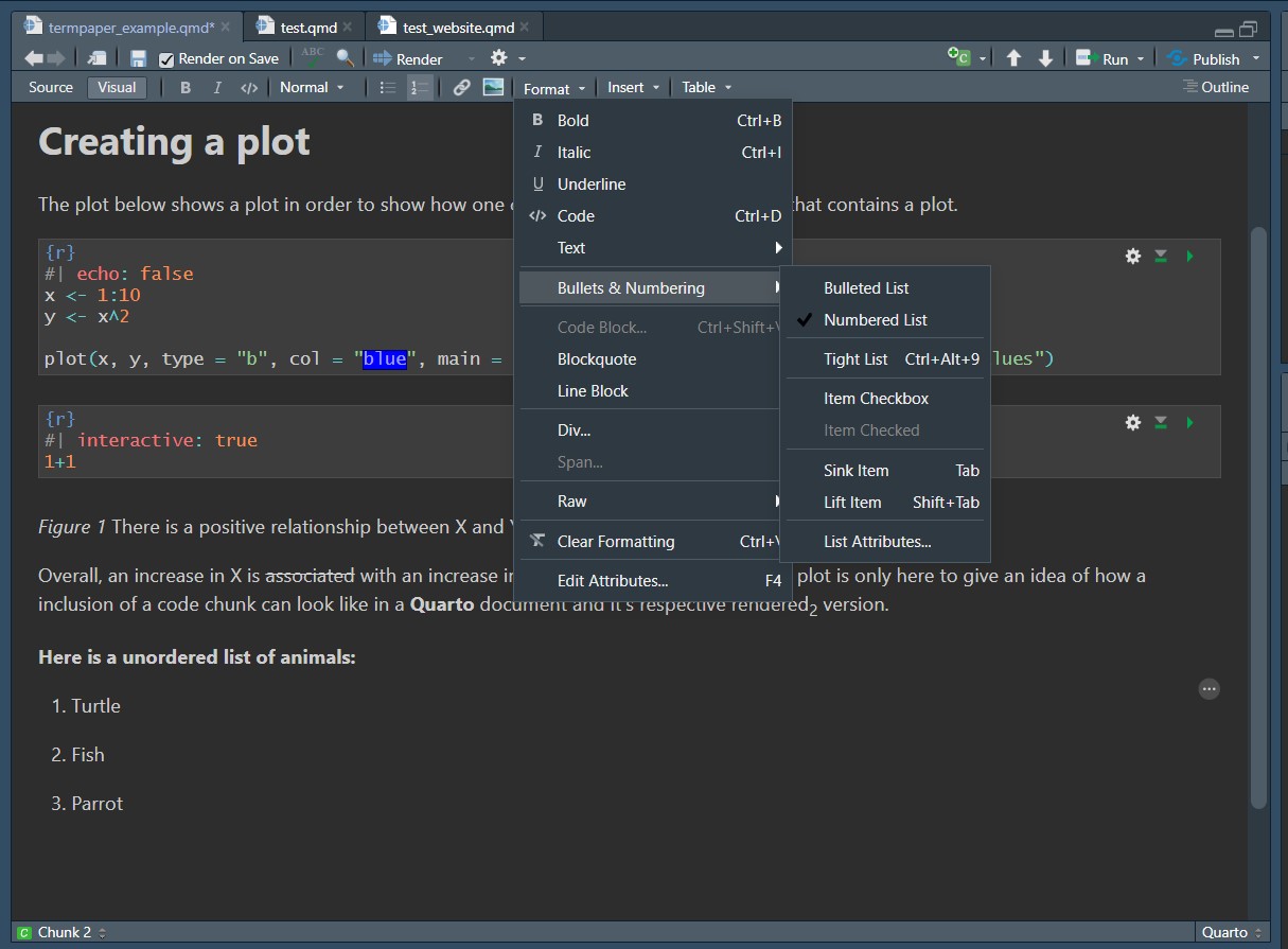
You have access to the same types of lists in the Visual as in the Source Editor. when wanting to create a list, head to the menu line under Format > Bullets & Numbering. Some of the options only become available once you’ve created a list and want to edit it, like Tight Listor Sink Item.
You can also create tables using Markdown. However, this is one case where using either the Visual Editor or even better a Markdown table creator is recommended. Doing this in the Source Editor is very tedious and in terms of speed will leave you hanging behind the Visual Editor. However, in case you want to give it a try or come across it in a Markdown document, take a look below at how to create a table in the Source Editor.
Each new line is also a new row in the table and the columns are created using | as separators. You can define the width of a column using - and define where the text should be centered using :. See below how to do this.
Input
| Right | Left | Default | Center |
|------:|:-----|---------|:------:|
|   12  |  12  |    12   |    12  |
|  123  |  123 |   123   |   123  |
|    1  |    1 |     1   |     1  |
Output
| Right | Left | Default | Center |
|---|---|---|---|
| 12 | 12 | 12 | 12 |
| 123 | 123 | 123 | 123 |
| 1 | 1 | 1 | 1 |
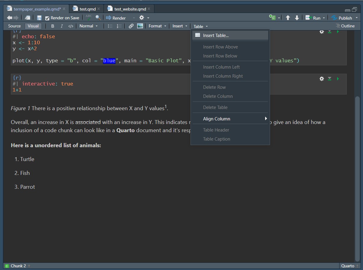
To create a table in the Visual Editor, head to the menu at the top again and go to Table > Insert Table…. This will open a prompt that asks you about the general dimensions of your table but you can still change these later on. You also have the option to include a caption at this point. Once you’ve created a table more options like centering or adding more rows will become available.
A very nice feature of Quarto is that it allows you to easily include equations. Regardless of which editor you use, you have to write the equations within LaTeX style. For a guide how to create sophisticated equations (including fractions, matrices, square roots, integrals, etc.), see the respective chapter in the LaTeX Beginner’s Guide.
To include an equation you need to frame it with dollarsigns $. One dollarsign for inline equations $ and two for a standalone equation $$.
As an example the input would like this:
Markdown
The most important equation remains `$E = mc^{2}$` up to this date.

The following equation remains the most important up to this date.

`$$E = mc^{2}$$`
And the respective outputs would look like this:
The most important equation remains \(E = mc^{2}\) up to this date.
The following equation remains the most important up to this date.
\[E = mc^{2}\]
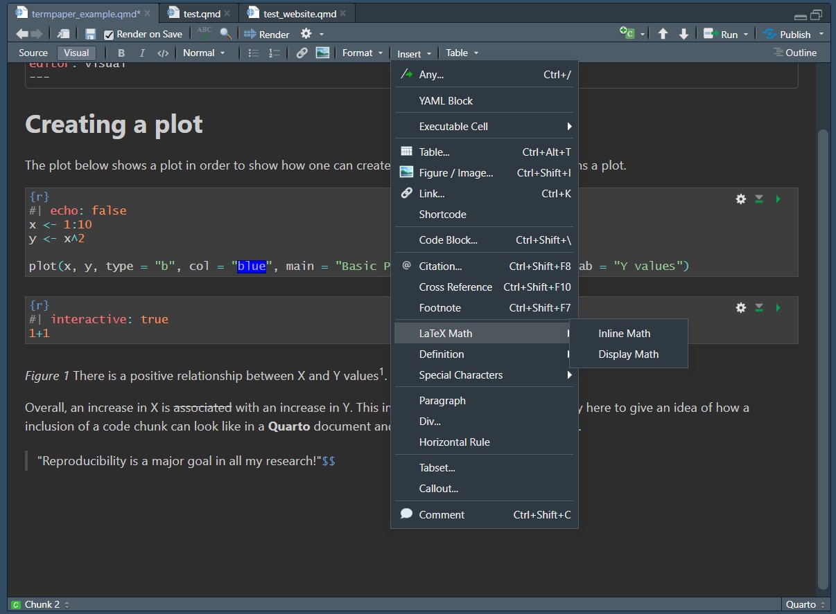
You can also add equations using the Visual Editor by going to the menu line and selecting Insert > LaTeX Math > Inline Math/Display Math.
You can insert blockquotes in your Quarto documents. Whilst this is likely not syntax you will need a lot in scientific reports, it’s very easy to do and might prove useful when taking notes or formatting a website you’re creating.
To create a blockquote in the Source Editor, just add a `<´before it.
For example you might want to insert a quote to emphasize your adoration for reproducibility and have this as your input.
> "Reproducibility is a major goal in all my research!"
This will result in the following output in your final document.
“Reproducibility is a major goal in all my research!”
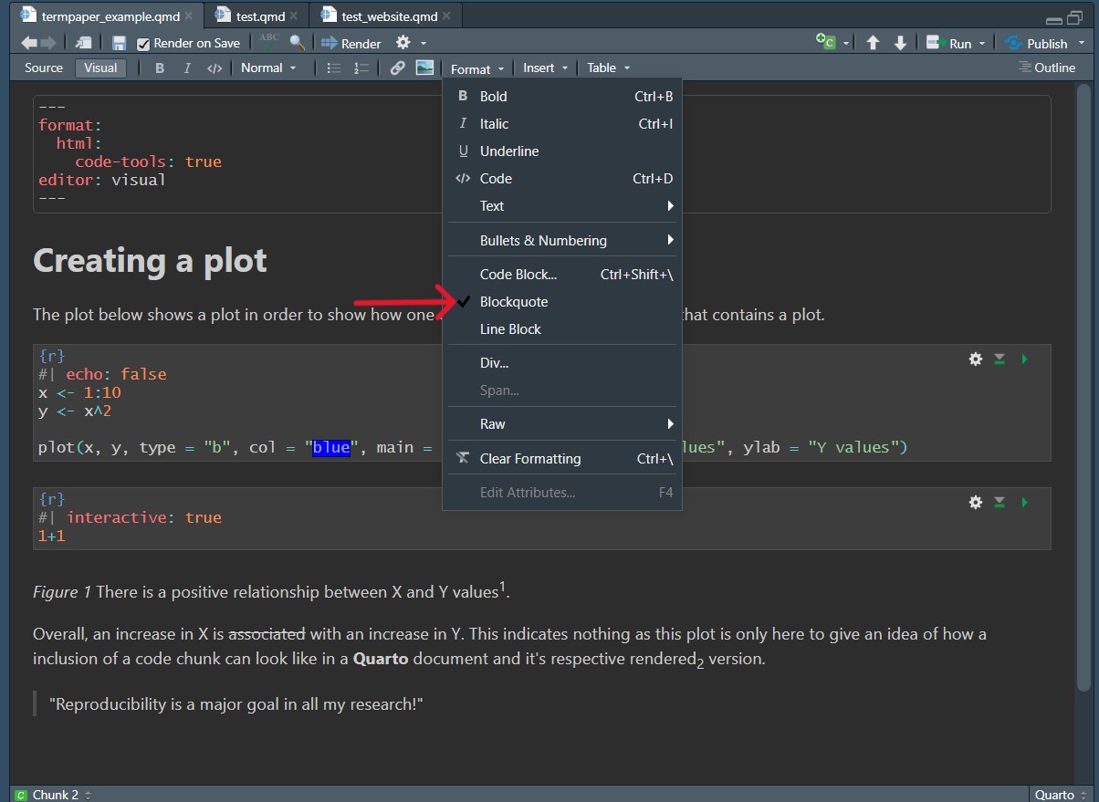
To do the same thing in the Visual Editor head once again to the menu line and select Format > Blockquote.
You can easily insert online links or images into your document. The process to do this is relatively similar, which is why the two actions are in the same section.
To insert a link to, for example a website, the most basic option is to just insert the link between angle brackets <Link>.
For example when referring to the Quarto website the input looks like this: <https://quarto.org/>.
And this results in this output: https://quarto.org/.
As this is maybe not the neatest way to insert a link, you can also “rename” the link by adding a custom name or description in square brackets [Name] and following this without a space in between with the link, this time in round brackets [Name](Link).
For our previous example, this looks like this as an input: [Quarto](https://quarto.org/)
And this is the resulting output: Quarto
Inserting an image works similarly. Let’s say you want to insert an image that you’ve found online, in this case the Quarto logo. To do this, start off with an exclamation mark, followed by squared brackets, which can contain a caption for your image, but you can otherwise leave empty, followed by the link to the image in round brackets .
For inserting the Quarto logo, this is the input:

Which will give you this output:

You can also add a link to your image. Staying with our Quarto example, here the Quarto logo will lead you to the Quarto website, but you could also use this process to link to your own website, a GitHub repository or your CV. The syntax for this is combining inserting an image and linking to something. Simply put the string used for inserting an image into squared brackets and follow this by the link in round brackets like so: [](Link).
For our example, this is the necessary input: [](https://quarto.org)
Resulting in this output (notice how clicking on the image will bring you to the Quarto websit):
You can of course also link to images you’ve taken yourself or that aren’t stored online by inserting a local image path instead of an online link. If the image is stored in the same subfolder as your document, you can refer to it directly, however it is recommended to create a designated image folder instead, to keep your project structure clear to others and your future self.
Let’s say your image quarto_logo.png is stored in the folder called images in a project structure like this:
| my-project.Rproj
| .gitignore
| README.html
| README.md
| code
| data
| images
  | quarto_logo.png
| renv
To insert it, your input looks like this: .
Returning you this output:
When using images or figures in e.g., a report about an analysis you’ve done, to not use a fixed image of it. Rather use a code chunk, which you will learn about in a little bit, to create it and keep them reproducible.
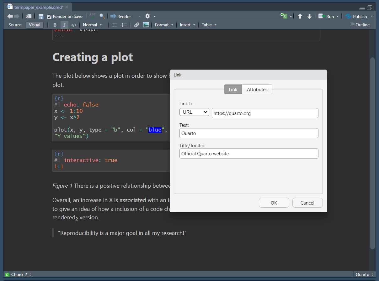
To add a link in the Visual Editor, head to the the menu line Insert > Link…, which opens a window that prompts you to enter the URL, a Text, which is what will be displayed within the text and a Title/Tooltip, which pops up when you hover over the link.
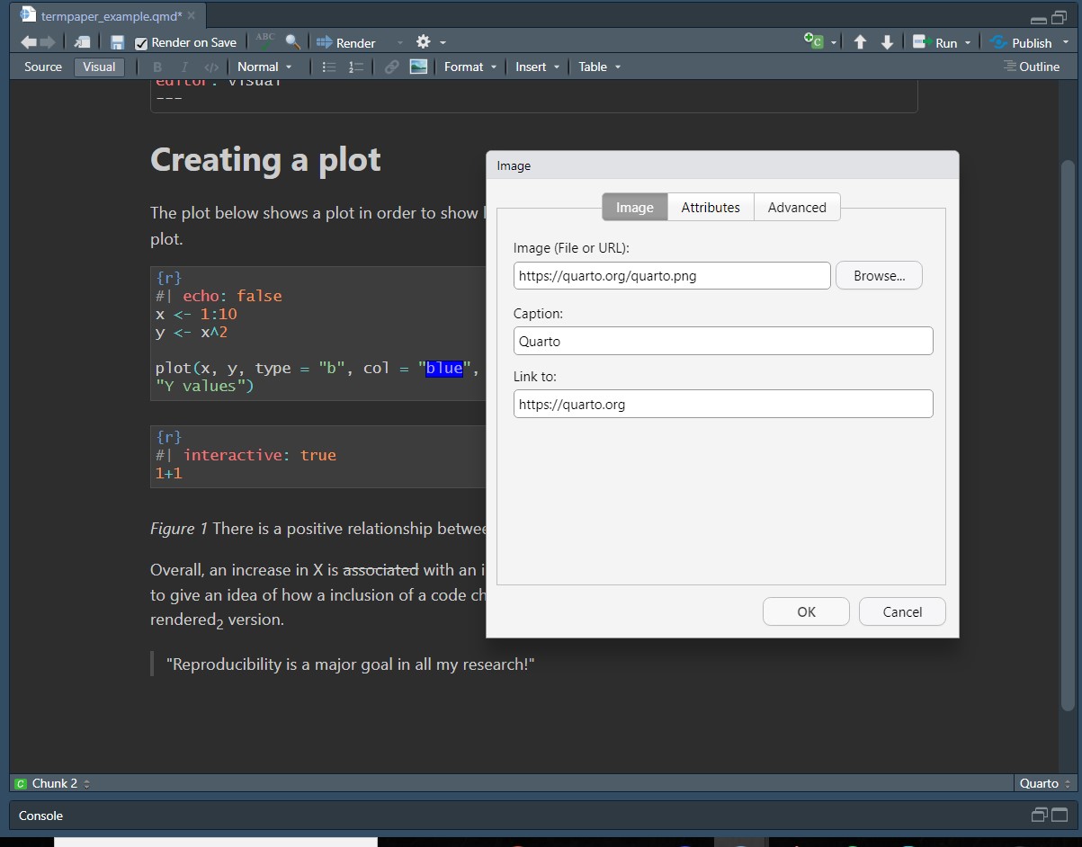
To insert images using the Visual Editor, select from the menu line Insert > Figure/Image…, which leads you to a pop-up window, in which you can either insert the link to an image or browse your stored images. In this window you can also add links to websites and a caption for your image.
In Quarto, every document starts with a YAML header. The YAML header is indicated by three hyphens (---) at the beginning and at the end (e.g. Figure 9.2 or Figure 9.4). After the YAML header, the document’s content begins.
YAML stands for Yet Another Markup Language. In the YAML header, you specify settings that belong to the whole document you are writing. In case, you want to write a book or create a website with Quarto, you will find a separate YAML file in your project directory (_quarto.yaml).
Do I need to learn another markup language? Good news is, YAML is really easy to learn. And in the context of Quarto, a comprehensive guide explains to you, how you can set up a variety of options for your quarto document. Thus, you do not really must learn YAML. When you do not know something, look at the guide and follow its instructions.
How is the setup of the YAML header? In general, the YAML header consists of so called key: value pairs. Thus, between the two lines with the three hyphens, you write (almost) everything in the style of a key that has a counterpart, called a value. key and value are separated by colon (:), while it comes directly after the key, but leaves one space open until the value starts. Each line only contains one key: value pair. When you use a string as a value, put quotation marks around the value (e.g. author: "Justus Reihs")
With the help of the key: value pairs, you can setup your whole Quarto document. You can specify the document’s title, name, published date, etc. It would take too much time to give you a comprehensive overview of YAML specifications. Hence, we will provide you an overview that shows you a) the most important specifications for when you write a paper and b) the most important specifications to keep that paper easy to reproduce.
| YAML key | Example | Description |
|---|---|---|
title |
|
Name the title of your document |
shorttitle shorttitle shorttitle |
|
The short title of your document |
author: |
|
The author(s) of your document and their affiliation(s) and address. You can include as many or as little of these pieces of information in your author description as you desire. |
editor |
|
Set that each sentence is placed in a new line (Tip 9.2) |
csl |
|
Set the citation style of your document |
` |
|
Refer to the citations you use in your document |
---
title: "Literate Programming"
editor: source
engine: knitr
execute:
  eval: false
  warning: false
  message: false
code-annotations: hover
categories: [intermediate]
abstract: |
  In this chapter you will learn how you can automatically integrate your reproducible results into a paper.
  You will learn how to write a paper in with Quarto and how to format it for a required output.
  You will learn how to use extension, specifically the apaquarto extension to write reproducible paper in APA-style.
---There are some nice features that can be implemented in Quarto, such as including code chunks, as mentioned before with the example of a plot, inline code, as well as referencing and citations. These are the features that can make your document reproducible. As explained in the introduction, when having to e.g. change your analysis, these features will update without you having to painstakingly change your results manually and likely introduce some errors in the process.
Code chunks are pieces of code that will be executed by Quarto during the rendering process, so when you’re having Quarto create the intended output format of your .qmd file. Remember the earlier example of a plot within a report, which was done using a code chunk.
Any type of code can be inserted by using code chunks.
To insert a code chunk either do so by using specific syntax in the Source mode or by going into the Visual mode and inserting it by clicking through the menu.
To add a code chunk in the Source mode, simply add three back ticks around your code and specify the language within {}. For example in the language R, this would look just like this: ```{r} Your code ```. As this process is so simply and the thinking work lies in the code itself, it is recommended to do this in the Source mode, also because it is simply faster.
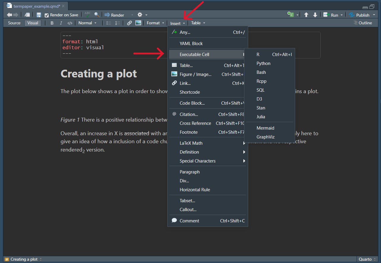
To add a code chunk in the Visual mode, head to Insert > Executable Cell > Desired Language , as can be seen below.
Code chunks can be quite different in their functioning. There is some room for how you can customize them, for example you might like to have the code displayed as well as the output or (very likely) you have a lot of code but only want to showcase your results directly in the output document but in order to get there you need to run a lot of code beforehand. As your biggest goal is keeping your document reproducible, you still want to include it in your Quarto file.
To do this, you use different Chunk Options. In the previous examples one of them has been #| echo: false, which ensures that only the output, in that case the plot, and not the input, the code is shown. To include them, place them within your code chunk, after your specified coding language, just like in the code chunk in the plot example above. The options are either specified trueor `false and prefaced by #|.
Some important options are:
- #| echo: false: When set to false, the code chunks results are shown but not the code itself. When set as true, the code is also shown.
- #| include: false: Neither the code nor the results appear in the output file, which is useful for code which’s results you need for running other code later on but isn’t relevant to the reader.
- #| warning: false: Don’t include potential warnings in the output.
- #| fig.cap = " Your caption": Include a caption in your figure. This one is not set to true or false but rather just the caption is included.
- #| label: You can give your code chunk a label to more easily identify the aim of this piece of code.
Inline code allows you to simply insert code as part of your other markdown syntax. This is especially useful for referencing analysis outputs. In keeping with reproducibility this ensures that if you change parts of your analysis, your results will update as well without you having to manually go into the text change them manually, risking that you might miss some. Furthermore, when writing your report, you don’t have to go back and forth, checking what your specific results were but instead can just refer to them and move on with writing.
To add inline code, it’s the same process as for inserting a code chunk but instead of three backticks, you just use one. Remember to include the programming language in {}.
The input could look something like this:
The number of observations is `{r} 8*20`.The programming language used here is R and this code will result in the output:
The number of observations is 160.
You can cross-reference objects like figures, tables or equations within your text. This is especially useful in reports when you need to refer to different figures. The references work as links to the objects and let you jump to them in the final document.
For example: Section 9.7.4 (@sec-citations) brings you to the section on citations in this book.
To be able to cross-reference tables, sections of your text, equations or figures, they need to have a label. You need to add the label after the inserted object. The label is in curly brackets and start with a hash # like so {#object-name}. For example, for an image this looks like this: {#fig-fish}. To reference it in the text you loose the curly brackets and replace the hash with an at-sign @, which looks like this As displayed in @fig-fish, this a fish..
Avoid using underscores _when creating your labels as this might cause problems when rendering to PDF. There is a set of predefined prefixes you can and should use to refer to your objects. Then just follow this with a name of your choosing.
| Type | Label Prefix |
|---|---|
| Figures | fig- |
| Tables | tbl- |
| Equations | eq- |
| Sections | sec- |
| Code listing | lst- |
| Theorem | thm- |
When you write a paper, you definitely must include citations. Quarto offers different ways of managing citations. We will give you an overview on how to handle them.
When you use citations in Quarto, you will definitely need a bibliography. This bibliography contains all the relevant information of your citations and is usually a BibLaTeX (.bib) or BibTeX (.bibtex) file. What you might optionally want to include, is a file that specifies the Citation Style Language. For more information on that, see Section 9.7.4.3.
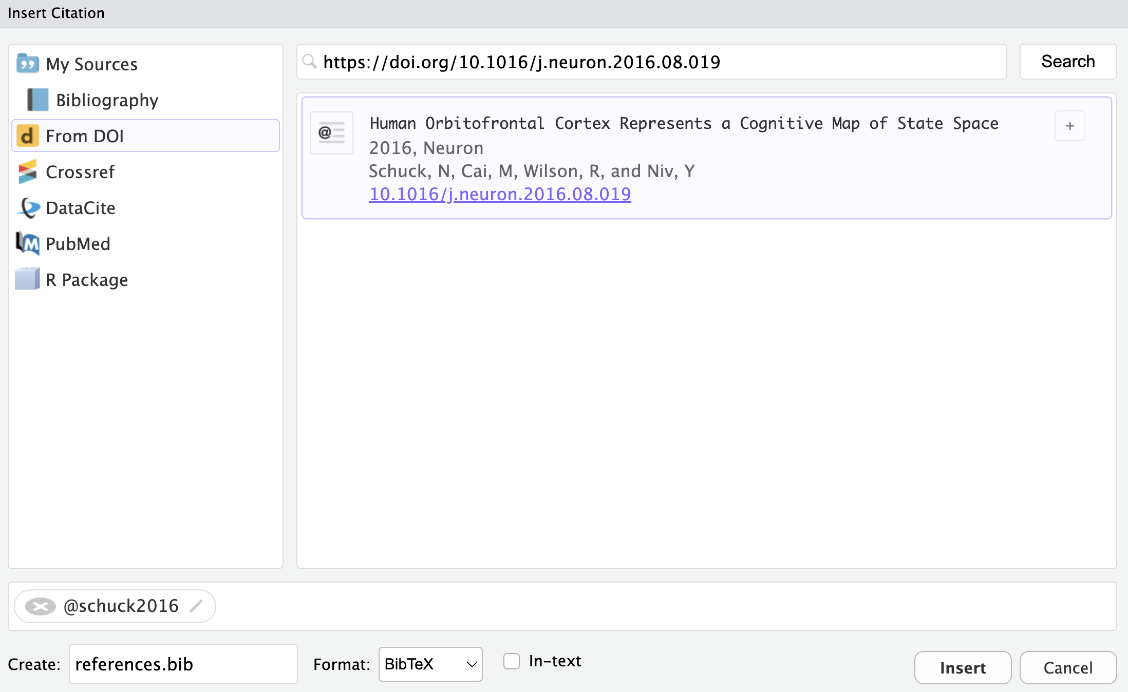
Adding citations is simple in the Visual Editor. Go to Insert in the menu line and click on Citation…. Then a box should pop up (see Figure 9.12). In that box, you have different options how to add a citation. In our opinion, the interface From DOI is the most convenient one for adding new citations. To find your citation of interest, simply copy and paste the DOI of your research article into the bar and hit Search. Then, your citation should be popped up in the pane below (again, see Figure 9.12). Simply hit Insert and your citation is in your document. At the same time (if it is your first citation), a references.bib file was automatically created in your project directory (see Note 9.2). Further, you can see, that your YAML header now contains one more line bibliography: references.bib. The Visual Editor does that automatically for you. If you use the Source editor, you have to set up the references.bib file on your own and manually add the bibliography key-value pair to your document’s YAML header. When you add other new citations, they are automatically added to your references.bib file, when you follow the same steps from above again.
references.bib file
The reference.bib file has a very specific setup. Lets look at an exemplary entry in the file to learn how it is built.
Example of `references.bib` file
@article{nuijten2024,
  author = {Michèle B. Nuijten and Jelte M. Wicherts},
  title = {Implementing Statcheck During Peer Review Is Related to a Steep Decline in Statistical-Reporting Inconsistencies},
  journal = {Advances in Methods and Practices in Psychological Science},
  year = {2024},
  volume = {7},
  issue = {2},
  doi = {10.1177/25152459241258945},
  url = {https://doi.org/10.1177/25152459241258945}
}
You can derive following rules from this example:
@@ the resource type of the entry is specified (e.g. article, book, etc.){ marks the begin of where to write the content of the citation{, an identifier is written (by default, first author name and the year of publication),, separates two key-value pairs, at the end} at a new line, closing the opening curly bracket from the first line of the entry.references.bib of this book.
references.bib
@article{knuth84,
  author = {Knuth, Donald E.},
  title = {Literate Programming},
  year = {1984},
  issue_date = {May 1984},
  publisher = {Oxford University Press, Inc.},
  address = {USA},
  volume = {27},
  number = {2},
  issn = {0010-4620},
  url = {https://doi.org/10.1093/comjnl/27.2.97},
  doi = {10.1093/comjnl/27.2.97},
  journal = {Comput. J.},
  month = may,
  pages = {97–111},
  numpages = {15}
}

@article{bakker2023,
  author = {Bakker, Arnold B. and Demerouti, Evangelia and Sanz-Vergel, Ana},
  title = {Job Demands-Resources Theory: Ten Years Later},
  issue_date = {January 2023},
  publisher = {Annual Review of Organizational Psychology and Organizational Behavior},
  volume = {10},
  url = {https://doi.org/10.1146/annurev-orgpsych-120920-053933},
  doi = {10.1146/annurev-orgpsych-120920-053933},
  journal = {Annual Review of Organizational Psychology and Organizational Behavior},
  month = jan,
  year = {2023},
  pages = {25-53},
  numpages = {29}
}

@inbook{goodhart1984,
    title = {Problems of Monetary Management: The UK Experience},
    author = {Goodhart, C. A. E.},
    year = {1984},
    date = {1984},
    publisher = {Macmillan Education UK},
    pages = {91--121},
    doi = {10.1007/978-1-349-17295-5_4},
    url = {http://dx.doi.org/10.1007/978-1-349-17295-5_4},
    langid = {en}
}

@article{mckiernan2016,
    title = {How open science helps researchers succeed},
    author = {McKiernan, Erin C and Bourne, Philip E and Brown, C Titus and Buck, Stuart and Kenall, Amye and Lin, Jennifer and McDougall, Damon and Nosek, Brian A and Ram, Karthik and Soderberg, Courtney K and Spies, Jeffrey R and Thaney, Kaitlin and Updegrove, Andrew and Woo, Kara H and Yarkoni, Tal},
    year = {2016},
    month = {07},
    date = {2016-07-07},
    journal = {eLife},
    volume = {5},
    doi = {10.7554/elife.16800},
    url = {http://dx.doi.org/10.7554/eLife.16800},
    langid = {en}
}

@article{abele-brehm2016,
    title = {Wer soll die Professur bekommen?},
    author = {Abele-Brehm, Andrea E. and {Bühner}, Markus},
    year = {2016},
    month = {10},
    date = {2016-10},
    journal = {Psychologische Rundschau},
    pages = {250--261},
    volume = {67},
    number = {4},
    doi = {10.1026/0033-3042/a000335},
    url = {http://dx.doi.org/10.1026/0033-3042/a000335},
    langid = {de}
}

@article{john2012,
    title = {Measuring the Prevalence of Questionable Research Practices With Incentives for Truth Telling},
    author = {John, Leslie K. and Loewenstein, George and Prelec, Drazen},
    year = {2012},
    month = {04},
    date = {2012-04-16},
    journal = {Psychological Science},
    pages = {524--532},
    volume = {23},
    number = {5},
    doi = {10.1177/0956797611430953},
    url = {http://dx.doi.org/10.1177/0956797611430953},
    langid = {en}
}

@article{nosek2022,
    title = {Replicability, Robustness, and Reproducibility in Psychological Science},
    author = {Nosek, Brian A. and Hardwicke, Tom E. and Moshontz, Hannah and Allard, {Aurélien} and Corker, Katherine S. and Dreber, Anna and Fidler, Fiona and Hilgard, Joe and Kline Struhl, Melissa and Nuijten, {Michèle B.} and Rohrer, Julia M. and Romero, Felipe and Scheel, Anne M. and Scherer, Laura D. and {Schönbrodt}, Felix D. and Vazire, Simine},
    year = {2022},
    month = {01},
    date = {2022-01-04},
    journal = {Annual Review of Psychology},
    pages = {719--748},
    volume = {73},
    number = {1},
    doi = {10.1146/annurev-psych-020821-114157},
    url = {http://dx.doi.org/10.1146/annurev-psych-020821-114157},
    langid = {en}
}

@misc{bryan2015,
  author = {Bryan, Jenny},
  title = {How to name files},
  year = {2015},
  month = {May},
  note = {[Online; accessed 19. Nov. 2020]},
  url = {https://speakerdeck.com/jennybc/how-to-name-files}
}

@book{chacon2014,
    title = {Pro Git},
    author = {Chacon, Scott and Straub, Ben},
    year = {2014},
    date = {2014},
    publisher = {Apress},
    doi = {10.1007/978-1-4842-0076-6},
    url = {http://dx.doi.org/10.1007/978-1-4842-0076-6},
    note = {License: CC BY-NC}
}
@article{hanson2019,
    title = {Data Sharing and Management Snafu in 3 Short Acts},
    author = {Hanson, Karen and Surkis, Alisa and Yacobucci, Karen},
    year = {2019},
    date = {2019},
    doi = {10.6084/M9.FIGSHARE.8061722.V1},
    url = {https://figshare.com/articles/Data_Sharing_and_Management_Snafu_in_3_Short_Acts/8061722/1}
}

@book{gau2022,
    title = {Remi-Gau/bids{\_}workshop: v0.1.1},
    author = {Gau, Remi},
    year = {2022},
    month = {10},
    date = {2022-10-09},
    publisher = {Zenodo},
    doi = {10.5281/ZENODO.7178587},
    url = {https://zenodo.org/record/7178587}
}

@article{wilkinson2016,
    title = {The FAIR Guiding Principles for scientific data management and stewardship},
    author = {Wilkinson, Mark D. and Dumontier, Michel and Aalbersberg, IJsbrand Jan and Appleton, Gabrielle and Axton, Myles and Baak, Arie and Blomberg, Niklas and Boiten, Jan-Willem and da Silva Santos, Luiz Bonino and Bourne, Philip E. and Bouwman, Jildau and Brookes, Anthony J. and Clark, Tim and Crosas, {Mercè} and Dillo, Ingrid and Dumon, Olivier and Edmunds, Scott and Evelo, Chris T. and Finkers, Richard and Gonzalez-Beltran, Alejandra and Gray, Alasdair J.G. and Groth, Paul and Goble, Carole and Grethe, Jeffrey S. and Heringa, Jaap and {{\textquoteright}t Hoen}, Peter A.C and Hooft, Rob and Kuhn, Tobias and Kok, Ruben and Kok, Joost and Lusher, Scott J. and Martone, Maryann E. and Mons, Albert and Packer, Abel L. and Persson, Bengt and Rocca-Serra, Philippe and Roos, Marco and van Schaik, Rene and Sansone, Susanna-Assunta and Schultes, Erik and Sengstag, Thierry and Slater, Ted and Strawn, George and Swertz, Morris A. and Thompson, Mark and van der Lei, Johan and van Mulligen, Erik and Velterop, Jan and Waagmeester, Andra and Wittenburg, Peter and Wolstencroft, Katherine and Zhao, Jun and Mons, Barend},
    year = {2016},
    month = {03},
    date = {2016-03-15},
    journal = {Scientific Data},
    volume = {3},
    number = {1},
    doi = {10.1038/sdata.2016.18},
    url = {http://dx.doi.org/10.1038/sdata.2016.18},
    langid = {en}
}

@article{gorgolewski2016,
    title = {The brain imaging data structure, a format for organizing and describing outputs of neuroimaging experiments},
    author = {Gorgolewski, Krzysztof J. and Auer, Tibor and Calhoun, Vince D. and Craddock, R. Cameron and Das, Samir and Duff, Eugene P. and Flandin, Guillaume and Ghosh, Satrajit S. and Glatard, Tristan and Halchenko, Yaroslav O. and Handwerker, Daniel A. and Hanke, Michael and Keator, David and Li, Xiangrui and Michael, Zachary and Maumet, Camille and Nichols, B. Nolan and Nichols, Thomas E. and Pellman, John and Poline, Jean-Baptiste and Rokem, Ariel and Schaefer, Gunnar and Sochat, Vanessa and Triplett, William and Turner, Jessica A. and Varoquaux, {Gaël} and Poldrack, Russell A.},
    year = {2016},
    month = {06},
    date = {2016-06-21},
    journal = {Scientific Data},
    volume = {3},
    number = {1},
    doi = {10.1038/sdata.2016.44},
    url = {http://dx.doi.org/10.1038/sdata.2016.44},
    langid = {en}
}

@article{broman2018,
  title = {Data Organization in Spreadsheets},
  author = {Karl W. Broman and Kara H. Woo},
  year = {2018},
  month = {04},
  date = {2018-04-24},
  journal = {The American Statistician},
  volume = {72},
  number = {1},
  pages ={2-10},
  doi = {10.1080/00031305.2017.1375989},
  url = {https://doi.org/10.1080/00031305.2017.1375989},
  langid = {en}
}

@article{wickham2014,
  title = {Tidy Data},
  author = {Hadley Wickham},
  year = {2014},
  month = {08},
  journal = {Jornal of Statistical Software},
  volume = {59},
  number = {10},
  pages = {1-23},
  doi = {10.18637/jss.v059.i10},
  url = {https://doi.org/10.18637/jss.v059.i10},
  langid = {en}
}

@Manual{fischetti2023,
  title = {assertr: Assertive Programming for R Analysis Pipelines},
  author = {Fischetti, Tony},
  year = {2023},
  month = {11},
  date = {2023-11-23},
  note = {R package version 3.0.1https://docs.ropensci.org/assertr/ (website)
https://github.com/ropensci/assertr},
  doi = {10.32614/CRAN.package.assertr},
  url = {https://docs.ropensci.org/assertr/},
}

@article{reinhart2010,
  author = {Reinhart, Carmen M. and Rogoff, Kenneth S.},
  title = {Growth in a Time of Debt},
  journal = {American Economic Review},
  volume = {100},
  number = {2},
  year = {2010},
  month = {May},
  pages = {573–78},
  doi = {10.1257/aer.100.2.573},
  url = {https://www.aeaweb.org/articles?id=10.1257/aer.100.2.573},
}

@article{herndon2014,
  title = {Does high public debt consistently stifle economic growth? A critique of Reinhart and Rogoff},
  author = {Thomas Herndon and Michael Ash and Robert Pollin},
  year = {2014},
  month = {03},
  journal = {Cambridge Journal of Economics},
  volume = {38},
  number = {2},
  pages = {257-279},
  doi = {10.1093/cje/bet075},
  url = {https://doi.org/10.1093/cje/bet075}
}

@article{ziemann2016,
  title = {Gene name erorrs are widespread in the scientific literature},
  author = {Ziemann, M. and Eren, Y. and El-Osta, A.},
  year = {2016},
  month = {08},
  date = {2016-08-23},
  journal = {Genome Biology},
  volume = {17},
  doi = {10.1186/s13059-016-1044-7},
  url = {https://doi.org/10.1186/s13059-016-1044-7}
}

@article{esteban2019,
  title = {fMRIPrep: a robust preprocessing pipeline for functional MRI},
  author = {Oscar Esteban and Christopher J. Markiewicz and Ross W. Blair and Craig A. Moodie and A. Ilkay Isik and Asier Erramuzpe and James D. Kent and Mathias Goncalves and Elizabeth DuPre and Medeleine Snyder and Hiroyuki Oya and Satrajit S. Gish and Jessey Wright and Joke Durnez and Russell A Poldrack and Krzysztof J. Gorgolewski},
  year = {2019},
  month = {01},
  journal = {Nature Methods},
  volume = {16},
  pages = {111-116},
  doi = {10.1038/s41592-018-0235-4},
  url = {https://doi.org/10.1038/s41592-018-0235-4}
}

@book{wittkuhn2024,
  author = {Lennart Wittkuhn and Konrad Pagenstedt},
  title = {Version Control Book},
  publisher = {ZFDM Repository},
  year = {2024},
  month = {02},
  doi = {10.25592/uhhfdm.14149},
  url = {https://doi.org/10.25592/uhhfdm.14149}
}

@book{wittkuhn2025,
  author = {Lennart Wittkuhn and Konrad Pagenstedt and Liese Kümmerle},
  title = {Version Control Book},
  year = {2025},
  month = {07},
  doi = {10.5281/zenodo.10724424},
  url = {https://lennartwittkuhn.com/version-control-book/}
}

@article{barker2022,
  author = {Barker, Michelle and Chue Hong, Neil P. and Katz, Daniel S. and Lamprecht, Anna-Lena and Martinez-Ortiz, Carlos and Psomopoulos, Fotis and Harrow, Jennifer and Castro, Leyla Jael and Gruenpeter, Morane and Martinez, Paula Andrea and Honeyman, Tom},
  title = {Introducing the FAIR Principles for research software},
  year = {2022},
  journal = {Scientific Data},
  volume = {9},
  pages = {622},
  doi = {10.1038/s41597-022-01710-x},
  url = {https://doi.org/10.1038/s41597-022-01710-x}

}

@book{wickham2023,
    title = {R for Data science: Import, Tidy, Transform, Visualize, and Model Data},
    author = {Wickham, H. and Çetinkaya-Rundel, M. and Grolemund, G.},
    year = {2023},
    data = {2023},
    publisher = {O'Reilly Media},
    url = {https://r4ds.hadley.nz},
    note = {License: CC BY-NC-ND 3.0 US}
}

@Manual{hester2024,
    title = {lintr: A 'Linter' for R Code},
    author = {Jim Hester and Florent Angly and Russ Hyde and Michael Chirico and Kun Ren and Alexander Rosenstock and Indrajeet Patil},
    year = {2024},
    note = {R package version 3.1.2},
    url = {https://CRAN.R-project.org/package=lintr},
}

@Manual{mueller2020,
    title = {here: A Simpler Way to Find Your Files},
    author = {Kirill Müller},
    year = {2020},
    note = {R package version 1.0.1, https://github.com/r-lib/here},
    url = {https://here.r-lib.org/},
  }

@misc{rennie2024,
  author       = {Nicola Rennie},
  title        = {Writing Better R Code},
  year         = {2024},
  url          = {https://nrennie.rbind.io/training-better-r-code/},
  note         = {Accessed on 2024-11-19}
}

@article{haslbeck2022,
  author = {Jonas M. Haslbeck and Oisín Ryan and Donald J. Robinaugh and Lourens J. Waldorp and Denny Borsboom},
  title = {Modeling Psychopathology: From Data Models to Formal Theories},
  year = {2022},
  journal = {Psychological Methods},
  volume = {27},
  issue = {6},
  pages = {930-957},
  doi = {10.1037/met0000303},
  url = {https://doi.org/10.1037/met0000303}
}

@Manual{ushey2024,
  title = {renv: Project Environments},
  author = {Kevin Ushey and Hadley Wickham},
  year = {2024},
  note = {R package version 1.0.11, https://github.com/rstudio/renv},
  url = {https://rstudio.github.io/renv/},
}

@misc{rapp2024,
  title = {Robust R Code That Will Work Forever With {renv}},
  url = {https://www.youtube.com/watch?v=Oen9xhEh8PY},
  journal = {YouTube},
  author = {Albert Rapp},
  year = {2024},
  month = {11},
}

@book{community2022,
    title = {The Turing Way: A handbook for reproducible, ethical and collaborative research},
    author = {{The Turing Way Community}},
    year = {2022},
    month = {07},
    date = {2022-07-27},
    publisher = {Zenodo},
    doi = {10.5281/zenodo.3233853},
    url = {https://zenodo.org/record/3233853},
    note = {License: \href{https://creativecommons.org/licenses/by/4.0/}{CC BY 4.0}. Source: \url{https://github.com/the-turing-way/the-turing-way}. Website: \url{https://the-turing-way.netlify.app/}}
}

@misc{wikipedia2025,
  title = {Modularity},
  url = {https://en.wikipedia.org/wiki/Modularity},
  author = {Wikipedia Contributors,},
  year = {2025},
  month = {02},
  day = {10}
}

@article{artner2021,
  title = {The Reproducibility of Statistical Results in Psychological Research: An Investigation Using Unpublished Raw Data},
  author = {Richard Artner and Thomas Verliefde and Sara Steegen and Sara Gomes and Frits Traets and Francis Tuerlinckx and Wolf Vanpaemel},
  year = {2021},
  journal = {Psychological Methods},
  volume = {26},
  issue = {5},
  pages = {527-546},
  doi = {10.1037/met0000365},
  url = {https://doi.org/10.1037/met0000365}
}

@article{crüwell2023,
  title = {What’s in a Badge? A Computational Reproducibility Investigation of the Open Data Badge Policy in One Issue of Psychological Science},
  author = {Sophia Crüwell and Deborah Apthorp and Bradley J. Baker and Lincoln Colling and Malte Elson and Sandra J. Geiger and Sebastian Lobentanzer and Jean Monéger and Alex Patterson and D. Samuel Schwarzkopf and Mirela Zaneva and Nicholas J. L. Brown},
  year = {2023},
  journal = {Psychological Science},
  volume = {34},
  issue = {4},
  pages = {513-522},
  doi = {10.1177/09567976221140828},
  url = {https://doi.org/10.1177/09567976221140828}
}

@article{hardwicke2021,
  title = {Analytic reproducibility in articles receiving open data badges at the Journal *Psychological Science*: an observational study},
  author = {Tom E. Hardwicke and Manuel Bohn and Kyle MacDonald and Emily Hembacher and Michéle B. Nuijten and Benjamin N. Peloquin and Benjamin E. deMayo and Bria Long and Erica J. Yoon and Michael C. Frank},
  year = {2021},
  journal = {Royal Society Open Science},
  volume = {8},
  pages = {201494},
  doi = {10.1098/rsos.201494},
  url = {https://doi.org/10.1098/rsos.201494}
}

@article{obels2020,
  title = {Analysis of Open Data and Computational Reproducibility in Registered Reports in Psychology},
  author = {Pepijn Obels and Daniël Lakens and Nicholas A. Coles and Jaroslav Gottfried and Seth A. Green},
  year = {2020},
  journal = {Advances in Methods and Practices in Psychological Science},
  volume = {3},
  issue = {2},
  pages = {229-237},
  doi = {10.1177/2515245920918872},
  url = {https://doi.org/10.1177/2515245920918872}
}

@article{lakomy2019,
  title = {Open Science and the Science-Society Relationship},
  author = {Martin Lakomý and Renata Hlavová and Hana Machackova},
  year = {2019},
  journal = {Society},
  volume = {56},
  pages = {246-255},
  doi = {10.1007/s12115-019-00361-w},
  url = {https://doi.org/10.1007/s12115-019-00361-w}
}

@book {cribb2010,
    author = {Julian Cribb and Tjempaka Sari},
    title = {Open Science: Sharing Knowledge in the Global Century},
    pages = {230},
    year = {2010},
    doi = {10.1071/9780643097643},
    publisher = {CSIRO Publishing},
    isbn = {978-0-643-10183-8},
    URL = {https://doi.org/10.1071/9780643097643}
}

@article{opensciencecollaboration2015,
  title = {Estimating the reproducibility of psychological science},
  author = {Open Science Collaboration,},
  year = {2015},
  month = {august},
  date = {2015-08-28},
  journal = {Science},
  volume = {349},
  pages = {aac4716},
  doi = {10.1126/science.aac4716},
  url = {https://doi.org/10.1126/science.aac4716}
}

@article{begley2012,
  title = {Raise standards for preclinical cancer research},
  author = {C. Glenn Begley and Lee M. Ellis},
  year = {2012},
  journal = {nature},
  volume = {483},
  pages = {531-533},
  doi = {10.1038/483531a},
  url = {https://doi.org/10.1038/483531a}
}

@article{stroop1935,
  title = {Studies of interference in serial verbal reactions},
  author = {Stroop, J. R.},
  year = {1935},
  journal = {Journal of Experimental Psychology},
  volume = {18},
  issue = {6},
  pages = {643-662},
  doi = {10.1037/h0054651},
  url = {https://doi.org/10.1037/h0054651}
}

@article{williams1996,
  title = {The emotional Stroop task and psychopathology},
  author = {Williams, J. M. G. and Mathews, A. and MacLeod, C.},
  year = {1996},
  journal = {Psychological Bulletin},
  volume = {120},
  issue = {1},
  pages = {3-24},
  doi = {10.1037/0033-2909.120.1.3},
  url = {https://doi.org/10.1037/0033-2909.120.1.3}
}

@article{poldrack2019,
  title = {The Costs of Reproducibility},
  journal = {Neuron},
  volume = {101},
  number = {1},
  pages = {11-14},
  year = {2019},
  issn = {0896-6273},
  doi = {https://doi.org/10.1016/j.neuron.2018.11.030},
  url = {https://www.sciencedirect.com/science/article/pii/S0896627318310390},
  author = {Russell A. Poldrack},
  abstract = {Improving the reproducibility of neuroscience research is of great concern, especially to early-career researchers (ECRs). Here I outline the potential costs for ECRs in adopting practices to improve reproducibility. I highlight the ways in which ECRs can achieve their career goals while doing better science and the need for established researchers to support them in these efforts.}
}

@misc{yarkoni2018,
  title = {No, it’s not The Incentives — it’s you},
  author = {Tal Yarkoni},
  url = {https://talyarkoni.org/blog/2018/10/02/no-its-not-the-incentives-its-you/},
  year = {2018},
  month = {October},
  day = {2},
  note = {Accessed: 2025-04-04}
}

@book{wagner2021,
  title        = {The DataLad Handbook},
  author       = {DataLad Community},
  year         = {2021},
  publisher    = {DataLad},
  url          = {https://handbook.datalad.org/},
  doi          = {https://doi.org/10.5281/zenodo.3608611},
  note = {License: \href{https://creativecommons.org/licenses/by-sa/4.0/}{CC BY-SA 4.0}. Source: \url{https://github.com/datalad-handbook/book?tab=License-1-ov-file}}
}

@article{laulie2023,
  title = {Exploring self-regulation theory as a mechanism of the effects of psychological contract fulfillment: The role of emotional intelligence},
  author = {Lyonel Laulié and Gabriel Briceño-Jiménez and Gisselle Henríquez-Gomez},
  year = {2023},
  journal = {Frontiers in Psychology},
  volume = {14},
  url = {https://www.frontiersin.org/journals/psychology/articles/10.3389/fpsyg.2023.1090094},
  doi = {10.3389/fpsyg.2023.1090094}
}

@article{nuijten2024,
  author = {Michèle B. Nuijten and Jelte M. Wicherts},
  title = {Implementing Statcheck During Peer Review Is Related to a Steep Decline in Statistical-Reporting Inconsistencies},
  journal = {Advances in Methods and Practices in Psychological Science},
  year = {2024},
  volume = {7},
  issue = {2},
  doi = {10.1177/25152459241258945},
  url = {https://doi.org/10.1177/25152459241258945}
}

@article{schuck2016,
    title = {Human Orbitofrontal Cortex Represents a Cognitive Map of State Space},
    author = {Schuck, {Nicolas W.} and Cai, {Ming Bo} and Wilson, {Robert C.} and Niv, Yael},
    year = {2016},
    month = {09},
    date = {2016-09},
    journal = {Neuron},
    pages = {1402--1412},
    volume = {91},
    number = {6},
    doi = {10.1016/j.neuron.2016.08.019},
    url = {http://dx.doi.org/10.1016/j.neuron.2016.08.019},
    langid = {en}
}

@misc{schoenbrodt2024,
  author = {Felix Schoenbrodt},
  title = {From the Replicability Crisis to Credible Science},
  year = {2024},
  url = {https://osf.io/652qw}
}

@misc{navarro,
  author ={Danielle Navarro},
  title = {Project Structure},
  url ={https://djnavarro.net/slides-project-structure/#1}
}

@misc{berd2023,
  author ={Academy, BERD},
  title = {BERD Course Booklet: Make Your Research Reproducible},
  year = {2023},
  url ={https://djnavarro.net/slides-project-structure/#1}
}

@software{quarto2025,
  author = {Allaire, J.J. and Teague, Charles and Scheidegger, Carlos and Xie, Yihui and Dervieux, Christophe and Woodhull, Gordon},
  month = apr,
  title = {Quarto},
  doi = {10.5281/zenodo.5960048},
  url = {https://github.com/quarto-dev/quarto-cli},
  version = {1.7},
  year = {2025}
}

@misc{wittkuhn2023,
  author = {Wittkuhn, Lennart},
  title = {Introduction to Quarto},
  license = {CC-BY-4.0},
  url = {https://github.com/lnnrtwttkhn/quarto-presentation/},
  version = {1.0},
  year = {2023}
}

@software{schneider2025,
  author = {Schneider, William Joel},
  title = {apaquarto},
  license = {CC0-1.0},
  year = {2025},
  url = {https://github.com/wjschne/apaquarto}
}To refer to citations that have already been inserted in your references.bib file, there is no difference between the Source and the Visual Editor. All you have to do is indicating a citation with @ and put the identifier (see Note 9.2) behind the @. Thus, if you want to cite the paper we added in Section 9.7.4.1, you can see in the references.bib file that we use the identifier schuck2016. Hence, the proper citation is @schuck2016. This citation is called an in-text citation. You can also use square brackets around the reference ([@schuck2016]). Another possibility is to use a - before the reference to let the authors disappear ([-@schuck2016]) Look at Table 9.2 to see how the different syntax plays out in the output.
| Markdown Format | Output (author-date format) |
|---|---|
|
Blip blop bloop (see Schuck et al. 2016, 33–35; also The Turing Way Community 2022, chap. 1) |
|
Blip blop bloop (Schuck et al. 2016, 1403–5, 1407–8 and passim) |
|
Blip blop bloop (Schuck et al. 2016). |
|
They say blah (2016) |
|
Schuck et al. (2016) says bloop. |
|
Schuck et al. (2016, 1403) says blah. |
By default, the citation style in Quarto Documents is the Chicago Manual of Style author-date format. If you want to change the style, you can look up different resources to find .csl files. These .csl files specify how the citations will be styled. Note 9.3 shows you some resources where you can find these .csl files.
To use the citation style language you downloaded with the .csl file, you have to make sure that the intended .csl file appears in the root directory of the project2. Additionally, make sure that you specified your YAML header by adding the key-value pair csl: apa.csl into the YAML header of your document (Tip 9.3).
One nice feature of Quarto are it’s extensions. These extensions are created from Quarto users to extend the behavior and functionality of quarto. Since Quarto contributes to the movement of Open Science and Reproducibility, these extensions are freely available.
apaquarto extensionIn this book, we will only deal with one extension - the apaquarto extension by William Joel Schneider. With this extension, we can shape the output of our rendered quarto file into the format of the APA guidelines3 without much effort.
To install apaquarto, there are some prerequisites that you most likely already fulfil.
Install Quarto
Install a programming language (e.g )
Install a programming environment (e.g. RStudio)
After you have installed all things, you can successfully install apaquarto. Most likely you have installed R and RStudio. To check whether Quarto is already installed, see Tip 9.4.
To check whether Quarto is already installed, open the Terminal at RStudio. It should be right next to the Console. If there is no Terminal, go to Tools > Terminal > New Terminal. Then, the Terminal pane will open. Write the following code into the Terminal:
Terminal
quarto --versionIf you already have Quarto installed, the current version of Quarto should be displayed.
Output
1.4.551If you have not installed Quarto yet, you might get a message like this:
Output
Command "quarto --version" not found.To install quarto, go head and follow the installation instructions at this website.
To install apaquarto, the installation guide offers multiple scenarios (see Tip 9.5). According to the guide, it is possible to install the extension from the Terminal and from the Console. However, in our experience, the console sometimes lead to errors, which is why we recommend to use the Terminal.
Steps to install the apaquarto extension:
Open your project folder in RStudio. In the folder you should write the Quarto document.
Go to the terminal in RStudio
Type the following command in the command line of the Terminal:
Terminal
quarto add wjschne/apaquartoOutput
Quarto extensions may execute code when documents are rendered.
If you do not trust the author of the extension,
we recommend that you do not install or use the extension.
? Do you trust the authors of this extension (Y/n) >Output
[✔] Downloading
[✔] Unzipping
          Found 1 extensions.

The following changes will be made:
My Document in APA Style, Seventh Edition    [No change]    (formats)
? Would you like to continue (Y/n) >Output
[✔] Copying
[✔] Extension installation complete

? View documentation using default browser? (Y/n) >apaquarto extension.When you now look at your project directory, you can see that a new folder exists called _extensions. In that folder, there is a subfolder called wjschne, which, in turn, contains a subfolder apaquarto. In that apaquarto subfolder, there are many files that constitute the settings for the apaquarto extension. We recommend not to change anything in this _extensions folder and all its subfolders manually.
apaquarto installation guide by William Joel Schneider
You now have the apaquarto extension installed, but when you render your Quarto document, it does not look like a document in APA style. A last (and simple) step is to change the YAML header of your Quarto document. You need to specify the format to be in apaquarto style. To do so write the code below into your YAML header, save the changes, and re-render your Quarto document.
YAML header
format:
apaquarto-docx: defaultapaquarto-html or apaquarto-pdf to render your .qmd file to a html or PDF file, respectively.
Now, your rendered Quarto document should be in APA style. However, R would not be R and Quarto would not be Quarto if there is a small detail to consider. This only works, when the Quarto document is placed in the same folder as the _extensions folder.
Make sure that your Quarto document (.qmd) is stored in the same folder as your _extensions folder!
Project Structure
.
| my-project.Rproj
| .gitignore
| README.html
| README.md
| apa-styled-quarto-document.qmd
| apa-styled-quarto-document.docx
| _extensions
  |-- wjschne
    |-- apaquarto
| code
| data
| renv
Above is displayed an excerpt of a project structure where the apaquarto extension works correctly. The .qmd-file is at the same folder as the _extensions folder.
Project Structure
.
| my-project.Rproj
| .gitignore
| README.html
| README.md
| apa-styled-quarto-document.qmd
| _extensions
  |-- wjschne
    |-- apaquarto
| code
| data
| report
  |--apa-styled-quarto-document.qmd
| renv
Above is displayed an excerpt of a project structure where the apaquarto extension does not work correctly. The .qmd-file is not at the same folder as the _extensions folder. Rather the .qmd file is located in the reports folder. Thus, the .qmd file is located on layer below the _extensions folder. Consequently, the apaquarto extension crushes when rerendering the Quarto document (which is why there is no .docx file in this project structure compared to the one that works correctly).
In case you are not completely flashed by these features of apaquarto (or you just do not have to submit your work in APA style), you might not need the apaquarto extension in your project and want to remove it. Despite dropping some tears, just type in the command below into your Terminal.
Terminal
quarto remove wjschne/apaquartoYou will get an output like this:
Output
? Are you sure you'd like to remove My Document in APA Style, Seventh Edition? (Y/n) >Type in Y and hit Enter. If you see the message below, you successfully deleted the extension form your project.
Output
Extension removed.We would like to express our gratitude to the following resources which have been essential in shaping this chapter. We recommend these references for further reading.
| Authors | Title | Website | License | Source |
|---|---|---|---|---|
| Allaire et al. (2025) | Quarto | MIT | ||
| Wittkuhn (2023) | Introduction to Quarto | CC-BY-4.0 | ||
| Schneider (2025) | Introduction to apaquarto | CCO-1.0 |
LaTeX is another markup language, such as markdown. To create PDF files from Quarto documents, you do not need to learn the markup language, but you need a LaTeX installation. To do so, follow the link displayed in Figure 9.3 (https://yihui.org/tinytex).↩︎
You can also put it in a subfolder of your project, but then you have to specify the path in the YAML header, too.↩︎
Many journals and universities require submissions to be in the APA format. Thus, we think it is useful for many students and researchers to know about this extension.↩︎